Experiments with Gabor features for learning time-frequency structured functions in low dimensional domains

Neural networks are well known to be universal function approximators, meaning roughly that for any not-too-badly-behaved function \( f \) and \(\varepsilon > 0\), we can find a neural network \( \mathcal{N} \) such that \( \Vert f - \mathcal{N} \Vert < \varepsilon\). However, the neural network \( \mathcal{N} \) might have to be unfeasibly large to approximate some functions. To mitigate this problem, we can first apply a feature mapping where instead of applying the neural network to the input coordinate \( \boldsymbol{x} \) directly, we apply some preprocessing \(F\) to \( \boldsymbol{x} \) and approximate the target function by \( \mathcal{N}(F(\boldsymbol{x}))\) instead. Specifically, we will be interested in feature mappings \( F \) that treat position (time) and frequency separately.

A natural question to ask is why one might wish to approximate a function representing an image, a signal, a video or a 3D model by a neural network. After all, the "standard" setting of a neural network is to map high dimensional data into either a few dimensions (classification, segmentation, object detection) or another high dimensional space (style transfer, denoising, point cloud completion). The two motivating settings closest to my heart are physics-informed neural networks (PINNs) and neural texture compression. In the former, we learn a function which should minimize a PDE loss functional and in the latter, made famous by the recent NVIDIA launch, we compress textures by expressing them as a neural network. In both of these cases, it is crucial that our networks are expressive in the sense that we can output functions without using too many parameters or epochs of training.

The most influential paper on this topic is the seminal 2020 paper Fourier Features Let Networks Learn High Frequency Functions in Low Dimensional Domains. In this post, we will go over some of the empirical insights from that paper and discuss an extension to a form of Gabor atoms.

Towards Fourier features

Machine learning methods are dependent on some source of non-linearity to be able to represent non-linear phenomena. We usually inject this in the form of the activation function. Still, without any further inductive bias, a network is likely to struggle to minimize losses which vary rapidly with the input. With the kernel method (kernel trick) we can gain appropriate nonlinearity by moving our inputs into a higher dimensional space where we believe our target function is likely to be easier to express. For example, to fit a simple ReLU MLP to a sine function, we would have to devote parameters to each of the many line segments which would make up the approximation. Applying a sine transformation of the input variable shortcuts this and opens the door to sparser representation of the data.

In Fourier analysis, we represent functions as sums of sines and cosines

The obvious way to utilize this relation for machine learning is perhaps to let the coefficients \( (\alpha_n)_n \) and \( (\beta_n)_n \) be the outputs of the neural network, i.e., \( \mathcal{N} : x \mapsto (\alpha_1, \dots, \beta_1, \dots) \). This is a viable approach but suffers from the fact that Fourier series are best suited for representing functions with a clear periodicity and non-varying frequency contents. Thus we might need a very large amount of terms to represent the function. Taking a step back and just noting that sines and cosines are expressive, we can choose them to be our features. This means, in the 1D case, that our feature map is

It turns out that picking the frequencies \( (a_n)_n,\, (b_n)_n \) randomly generally works, although they should be of comparable sizes to the Fourier series of the target function. Then combinations of these terms afford us greater freedom than just linear combinations of them.

We now try this out on a simple example of a chirp function, meaning a sinusoidal function with increasing frequency. Our MLP is standard and for the Fourier feature mapping we will use the following class.

class FourierFeatureMapping(nn.Module):
    def __init__(self, input_dim, num_features=16, sigma_freq=20.0, trainable=False):
        super(FourierFeatureMapping, self).__init__()
        freqs = torch.randn(input_dim, num_features) * sigma_freq
        if trainable:
            self.freqs = nn.Parameter(freqs)
        else:
            self.register_buffer('freqs', freqs)

    def forward(self, x):
        projection = 2 * np.pi * (x @ self.freqs)
        return torch.cat([torch.cos(projection), torch.sin(projection)], dim=-1)
	

Note that this code works for higher dimensions and that we have a flag for if the frequencies should be trainable or fixed. Now training this, together with an MLP with 3 hidden layers, all of dimension 256, we get the following progress over the epochs.

This problem is easy enough that we don't need to learn the Fourier coefficients but not having to rely on them being appropriate a priori means we're less dependent on hyperparameter tuning. If we would have chosen a smaller network, the Fourier features would still be able to learn the function but the naive method would struggle even more. For no feature mapping, the low-frequency bias of the output is clearly visible.

Adding localization

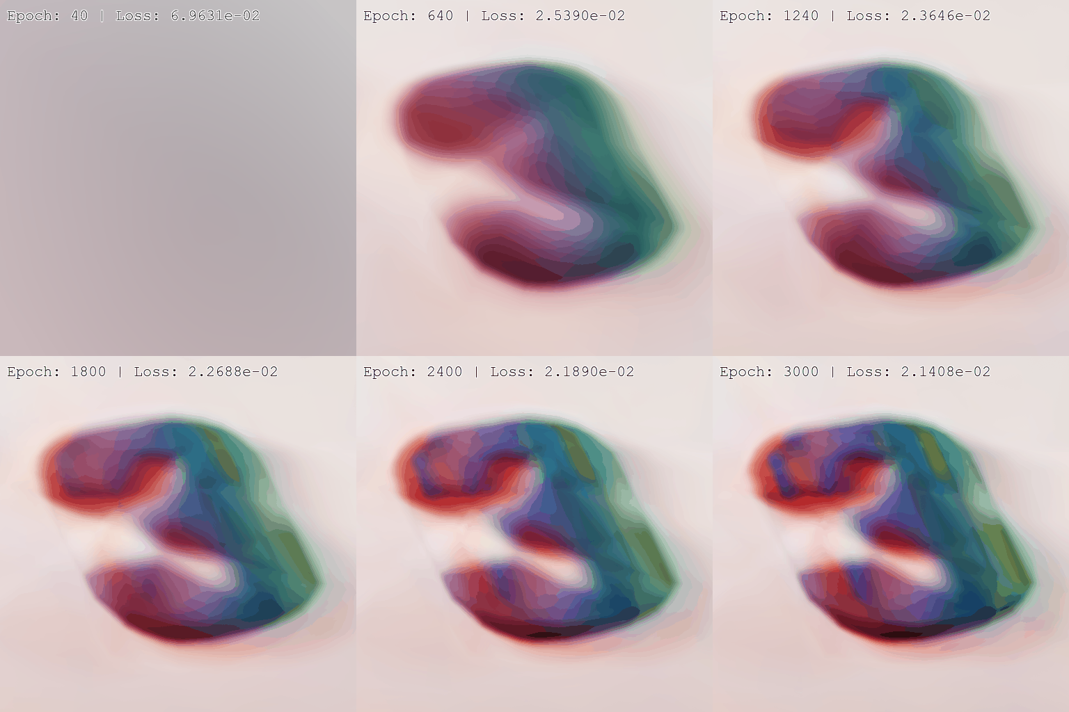
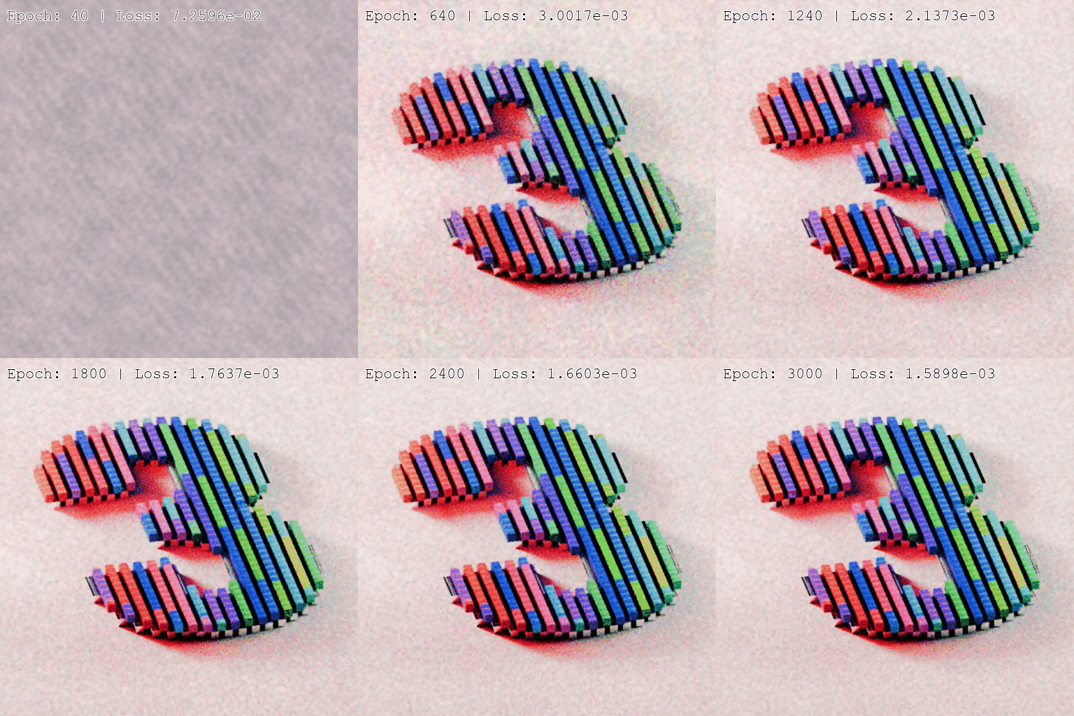
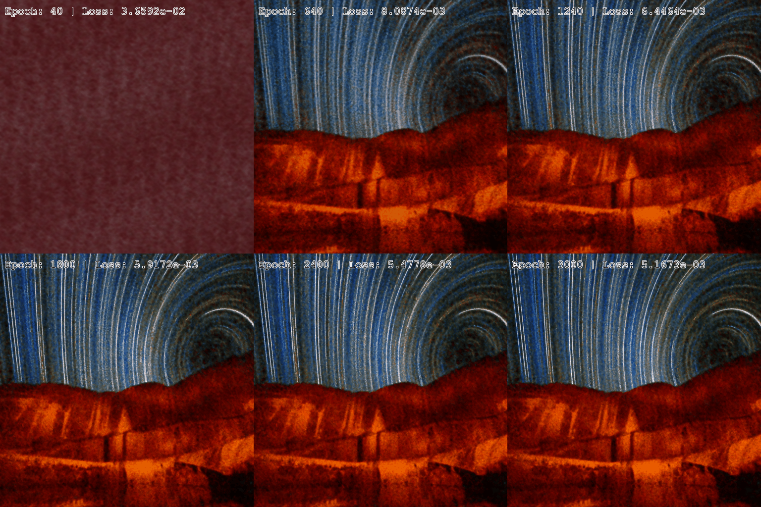
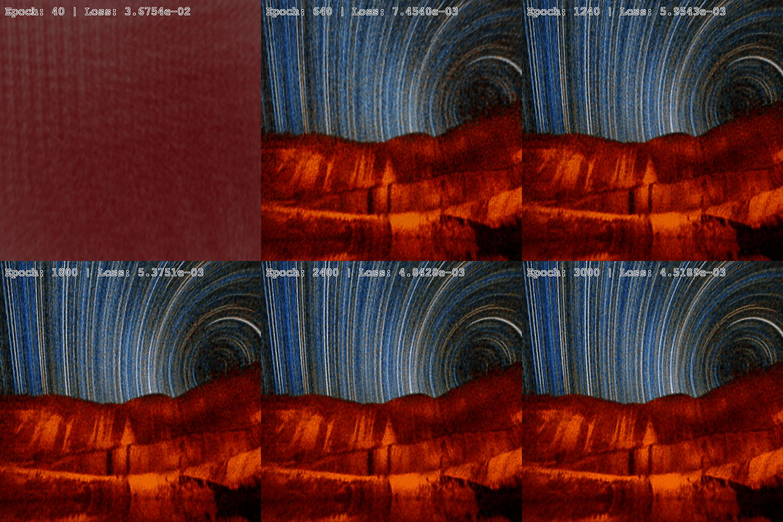
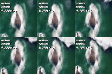
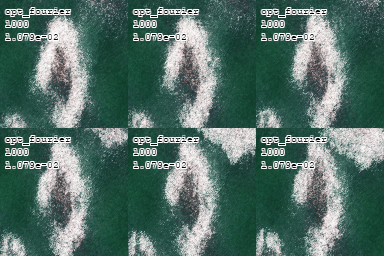
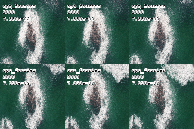
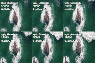
Fourier features clearly are very powerful and a staple of the field. Looking at weaknesses from a time-frequency perspective though, the standard argument against using tools based on Fourier series is that if I want to represent non-smooth and highly localized data I will need to use very high frequency building blocks. These building blocks are then hard to cancel out, resulting in noise. For an example of this, look at the uneven background in the middle image of the first figure of this post.

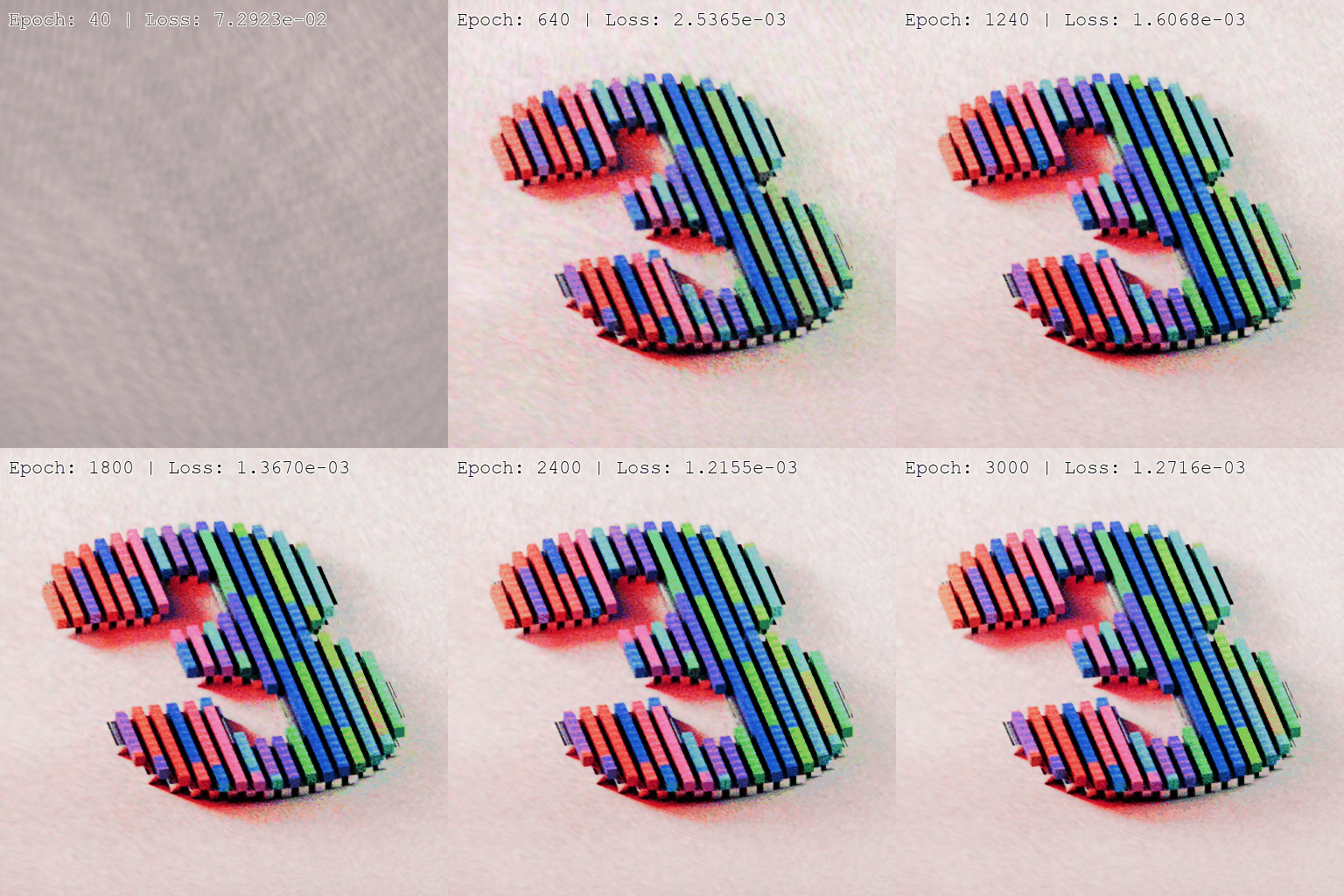
To circumvent this problem, we can consider sinusoids which are localized in the input space through modulated Gaussians of the form \( e^{-|x-c|^2/\sigma^2}\sin(\omega x) \). Now we have three parameters instead, the center \( c \), the width \( \sigma \) and the frequency \( \omega \). For a fixed \( \sigma \), we would call this a Gabor atom in time-frequency analysis. The point is that we can use different frequencies at different parts of the input space instead of sinusoids which span the entire input. In the example at the top, we have the same number of features and the same number of parameters in our MLP yet the loss is lower with the Gabor feature mappings.

Setting up this feature mapping is similar in nature to the FourierFeatureMapping example earlier. We initialize the centers in the interval \( [0,1] \) and make sure to transform our data to this domain beforehand and initialize all the widths as 0.1

class GaborFeatureMapping(nn.Module):
    def __init__(self, input_dim, num_features=16, sigma=0.1, sigma_freq=20.0, trainable=False):
        super(GaborFeatureMapping, self).__init__()
        
        centers = torch.rand(num_features, input_dim)
        frequencies = torch.randn(num_features, input_dim) * sigma_freq
        sigmas = torch.full((num_features, input_dim), sigma)

        if trainable:
            self.centers = nn.Parameter(centers)
            self.frequencies = nn.Parameter(frequencies)
            self.sigmas = nn.Parameter(sigmas)
        else:
            self.register_buffer('centers', centers)
            self.register_buffer('frequencies', frequencies)
            self.register_buffer('sigmas', sigmas)

    def forward(self, x):
        diff = x.unsqueeze(1) - self.centers.unsqueeze(0)
        envelope = torch.exp(- (diff ** 2 / (self.sigmas.unsqueeze(0) ** 2)).sum(dim=2) / 2)
        phase = 2 * np.pi * (diff * self.frequencies.unsqueeze(0)).sum(dim=2)
        cos_part = envelope * torch.cos(phase)
        sin_part = envelope * torch.sin(phase)
        return torch.cat([cos_part, sin_part], dim=-1)
	

We try this mapping out on another image which has a good mixture of low- and high-frequency details below with 48 features, 3 layers and a hidden dimension of 128.

It is worth stressing that we use the same number of Fourier features as Gabor features and so the computational load of these methods are comparable. In testing for this example and others, we have seen that setting Fourier features parameters as trainable is not always beneficial while for Gabor features this seems to always be the case. This is most likely because the Gabor transform of an image is likely to be sparser than its Fourier transform.

Video data

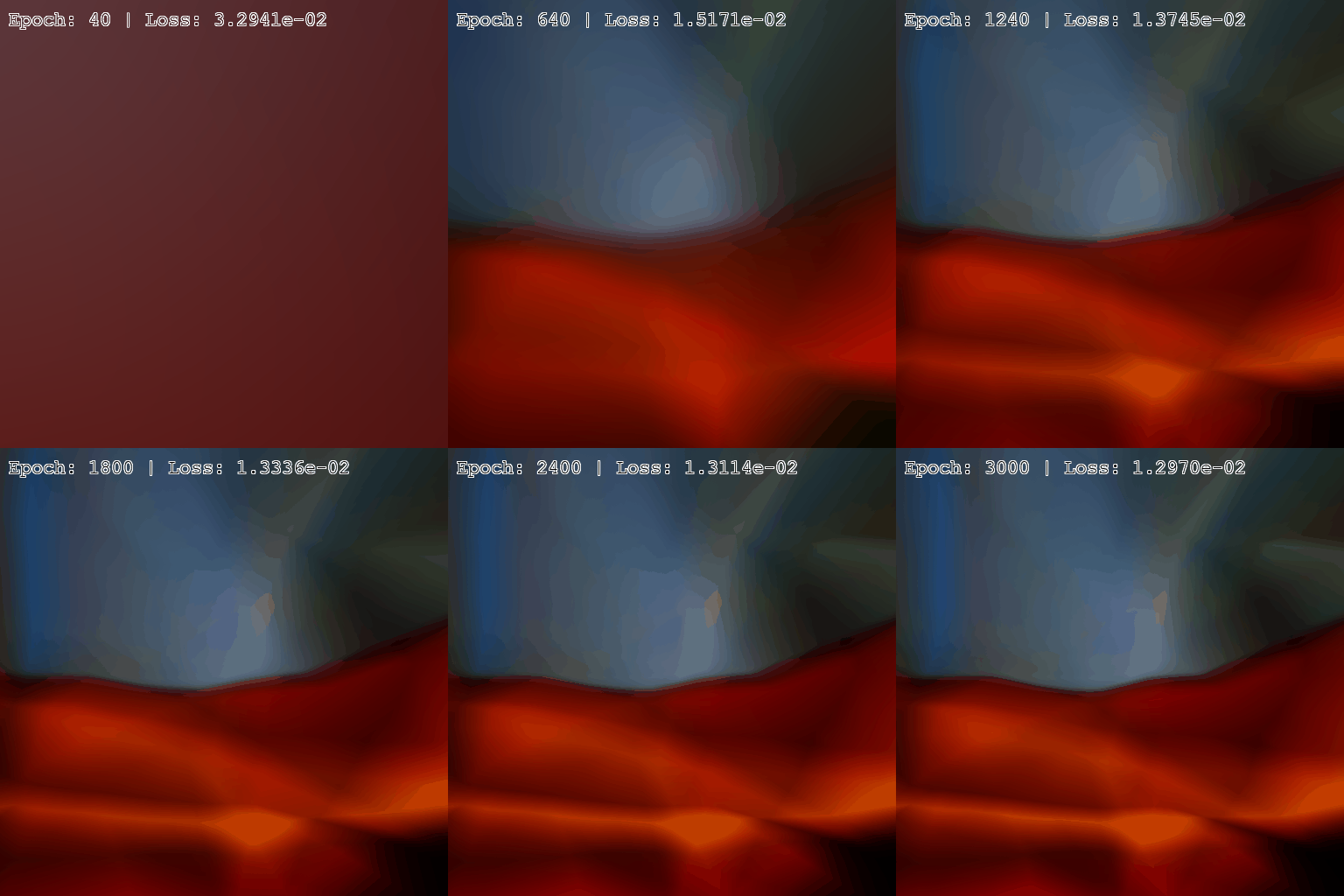
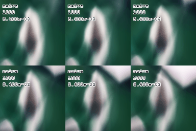
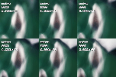
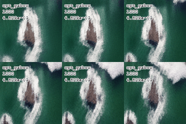
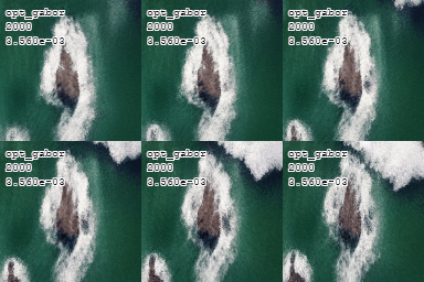
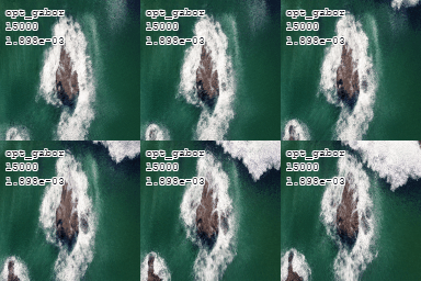
Lastly we will take a look at expressing a video, i.e. a function \( (x, y, t) \mapsto (r, g, b) \) in this manner. The idea is to really challenge the network. In the example below, we use 64 features and an MLP with 3 hidden layers, each of dimension 256. We downsample the video to be 128 x 128 to save on runtime.

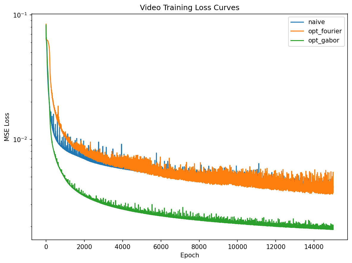
In this example the Gabor features perform substantially better than the Fourier features and the issue with noise for the Fourier features is very pronounced. In the loss curve below this phenomenon is quantified.

In a way, the network can be seen as a (lossy) video encoding scheme. Combining the learnable feature mapping with an MLP means that we can tune where in the encoding we want to place our parameters. This particular video example has parameters taking up around 260 kB with fp16. This is smaller than the original video file with no compression but still very lossy. Still, it speaks to the expressiveness of networks of this type, especially for PINN applications.

Conclusion

We have seen how we via a rather simple change can improve the standard Fourier feature mapping, especially for more complicated data. Apart from the code blocks in this post, the code to generate all the figures is standard boilerplate. Without more ablation studies and examples in different domains we cannot draw too strong conclusions but the point has been more to confirm the value of the general idea of using features from time-frequency analysis for these types of problems.

The code for all the figures in this post can be found here.