Five minute LLMs

Over the past few years there have been many innovations in LLM design: smart pretraining recipes, substantial post-training RL, and architectural improvements. In this post, we'll look at how some of the architectural improvements translate to very small models trained for short amounts of time. This means that we are not optimizing for low parameter count, the optimal choice there would be something like Gemma 3 270M. We are also not interested in distillation nor quantization. Instead, we are interested in the optimal design choices when training a model for only five minutes with consumer hardware on a smaller dataset. The recent exploration What's the strongest AI model you can train on a laptop in five minutes? by Sean Goedecke inspired this post and here we will aim to go deeper in terms of optimizing the architecture and doing proper A/B testing. The ultimate form for this type of investigation is Modded-NanoGPT which is considerably more hardcore but less accessible.

Following the post by Goedecke, we will restrict ourselves to the TinyStories dataset and pick validation cross-entropy as the metric which we are ultimately optimizing for. We will start from a GPT-2 style model and look at the effect of the following choices:

• Learning rate
• Schedule-Free optimizer
• Model sizing (hidden dimension, layers, heads)
• Gradient clipping
• FFN: MLP/SwiGLU
• Dropout
• Pre/post norm
• LayerNorm/RMSNorm
• Sinusoidal/learnable positional embeddings

What we change

This excellent overview by Sebastian Raschka looks at some of the ways modern models differ from the classical GPT-2 model. There is an overwhelming amount of papers suggesting various changes to the base transformer architecture, and through the test of time what is considered "standard" has evolved considerably. Below we briefly outline some of those developments which we vary in this post.

Schedule-Free

Introduced in the 2024 The Road Less Scheduled paper, the Schedule-Free optimizer from Meta promises to outperform the standard AdamW optimizer without the need for a complicated cosine scheduler. Removing the need for a scheduler or, alternatively, getting some of the benefits of a scheduler without the need to add additional hyperparameters sounds like a very nice deal. I've used this for some projects before and the results in the paper for a ResNet and an LLM are promising so I wanted to try it out here.

Usage is quite simple but not quite a drop-in replacement. Initialization is standard but we need to keep track of an internal train/eval mode just like we toggle for model during training/inference.

import schedulefree

...

if args["optimizer"] == "adamw":
	optimizer = torch.optim.AdamW(model.parameters(), lr=args["lr"])
else:
	optimizer = schedulefree.AdamWScheduleFree(model.parameters(), lr=args["lr"])

...

if args["optimizer"] == "schedulefree" and optimizer is not None:
	if train:
		optimizer.train()
	else:
		optimizer.eval()

Gradient clipping

Gradient clipping is a popular technique to stabilize training by clipping large gradients, avoiding particularly large gradients which may steer training off its course. In between loss.backward() and optimizer.step() we simply call nn.utils.clip_grad_norm_(model.parameters(), args["grad_clip"])

SwiGLU

In the latter part of a transformer block is a feedforward network (FFN) which originally took the form of a standard multilayer perceptron (MLP) with ReLU activation. In the years since, the Swish (also called SiLU) activation function has grown in popularity and the FFN has been modified to incorporate Gated Linear Units (GLUs). The original paper GLU Variants Improve Transformer by Noam Shazeer contains extensive tests on older architectures but modern LLMs seem to all include this modification.

class SwiGLU(nn.Module):
    def __init__(self, d_model: int, hidden: int, dropout: float):
        super().__init__()
        self.fc1 = nn.Linear(d_model, 2 * hidden)
        self.fc2 = nn.Linear(hidden, d_model)
        self.drop = nn.Dropout(dropout)

    def forward(self, x):
        u, v = self.fc1(x).chunk(2, dim=-1)      # [*, 2*hidden] -> two [*, hidden]
        x = F.silu(u) * v                         # SwiGLU: swish(u) ⊙ v
        x = self.fc2(x)
        return self.drop(x)

Dropout

Dropout is a very old (by modern standards) regularization technique. I feel like I've read papers both positive and negative about dropout in LLMs but the prevailing notion seems to be that it is superfluous, especially since we rarely train for high numbers of epochs in today's era of high parameter counts.

RMSNorm

LayerNorm is the standard solution for normalizing the state tensor over the feature dimension while going through transformer blocks by subtracting the mean, dividing by the standard deviation and applying a learned affine map. In RMSNorm, we skip the subtracting of the mean, allowing activations to drift more. As I've understood it, this minor change slightly improves throughput while having an even lesser effect on performance of the models. Both LayerNorm and RMSNorm are standard enough nowadays to be included in PyTorch as nn.LayerNorm and nn.RMSNorm.

Pre/post norm

Vanishing gradients have for a long time been a problem for deep networks. Apart from skip connections, the original Vaswani transformer paper also included two normalization layers inside each transformer block to stabilize training. These normalizations were placed after the attention and feedforward networks but later work has largely placed this part before each sub-block.

Sinusoidal/learnable positional embeddings

Sinusoidal positional embeddings were used in the original transformer paper but were quickly replaced by learned embeddings and later Rotary Positional Embeddings (RoPE). While RoPE acts directly on the Q and K matrices, sinusoidal and learned positional embeddings simply take the form of adding a vector to each token embedding making them a bit easier to implement.

Methodology

We will train all models with automatic mixed precision (AMP) and bfloat16 since this generally doubles throughput at the cost of some training stability which is preferable in this time-constrained setting. Everything will be run on an RTX 3070 with a context window of 256 tokens and a batch size of 16. Searching over all possible configurations is outside my time and electricity budget so we will assume that all choices contribute to the result independently.

args = {
		"lr":			2e-3,
        "optimizer":    "adamw",
        "n_layer":      2,
        "n_head":       2,
        "d_model":      128,
        "dropout":      0.0,
        "grad_clip":    None,
        "norm":         "layer",
        "ffn":          "mlp",
        "prepost":      "pre",
        "pos_emb":      "sinusoidal"
}

The performance of our models will have natural variation. To be able to conduct meaningful A/B experiments, we need to have a model for how our metric naturally varies. We can investigate this manually by constructing a histogram of validation cross-entropy for our default configuration.

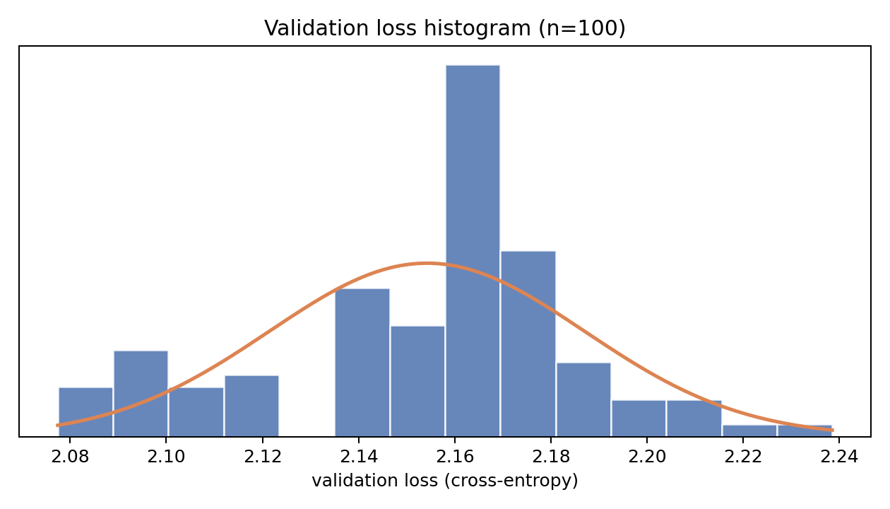
As we (hopefully) see in the figure, this distribution is at least somewhat Gaussian. For a given configuration, we will want to estimate the mean of the probability distribution which validation cross-entropy for models trained with this distribution follows. Since we do not know the variance, we will model our estimate for the true mean using the Student's $t$-distribution. Using this distribution, we can get confidence intervals for the true mean as $$ \bar{x} \pm t_{1-\alpha/2,\, n-1} \frac{s}{\sqrt{n}} $$ where $\bar{x}$ is the sample mean, $s$ is the sample standard deviation, $n$ is the number of samples and $\alpha$ is the parameter for the confidence interval.

From here, we will tweak the architecture to beat this base validation loss of around 2.15. Going over all possible configurations is simply infeasible, even on a 5 minute time budget, without significant parallel compute. Instead, we will work through the hyperparameters in a semi-heuristic way, tweaking the most important parameters first.

Hyperparameter search

As our first course of action, we will sweep over the learning rate between 1e-4 and 1e-2 for both AdamW and Schedule-Free AdamW since this hyperparameter can have a large effect. Doing this we find the following behavior:

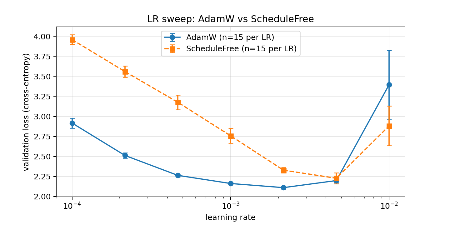
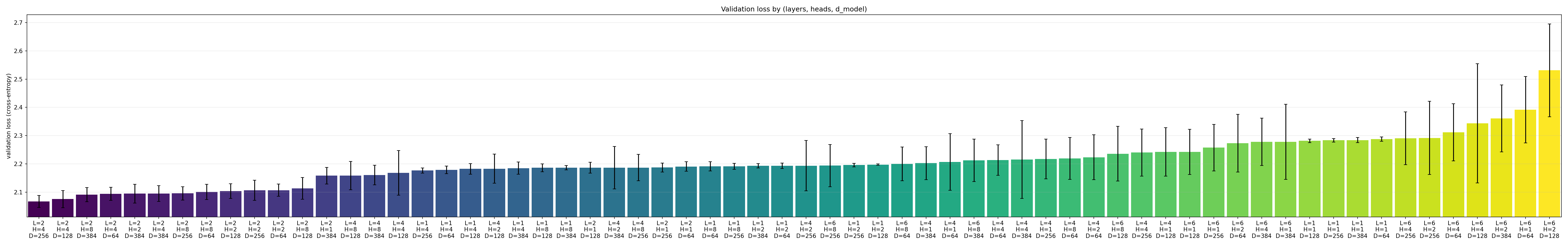
Based on this information, we set our configuration's learning rate to 2e-3 and stick with the standard AdamW optimizer. Next up we tweak the scaling hyperparameters for the model, the number of layers n_layers, the number of heads n_heads and the hidden model dimension d_model. Tweaking all of these at the same time for four different options for each hyperparameters means going over 4 × 4 × 4 = 64 configurations with several runs for each to develop confidence intervals.

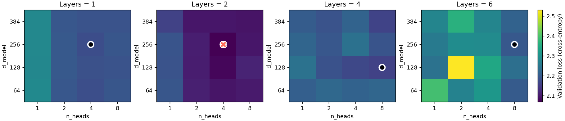
Running these sweeps is time intensive due to the large search space so we only perform 7 training runs per configuration. Still we can see continuity in the heatmaps above.

Note that we cannot say with any $p < 0.05$ confidence that the n_layers=2, n_heads = 4, d_model = 256 configuration is the global minimum in our search space but it is clear from the heatmaps that it at least is very close to the global minimum and so we set it in our configuration for now. Next up we compare RMSNorm and LayerNorm.

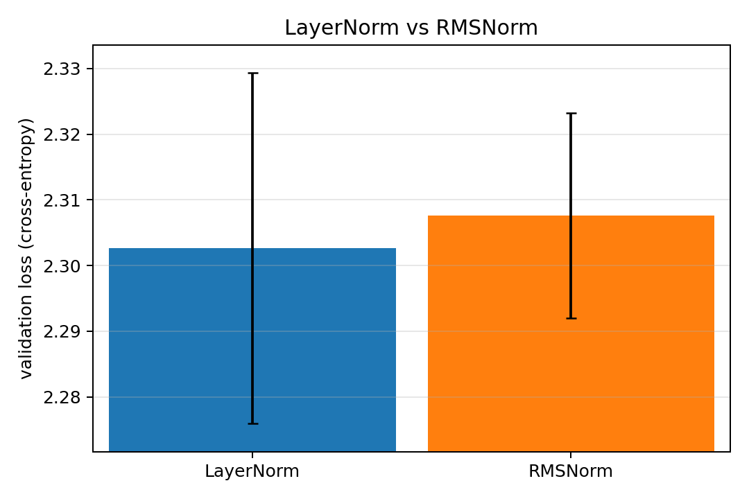
As we see in the figure, there is no clear winner despite this being the averages over 80 training runs per configuration. This is however to be expected as the optimization in RMSNorm is so small that it should only make a difference for much larger networks. Nevertheless, it is good to know that its simplification does not derail training for small sizes and training times.

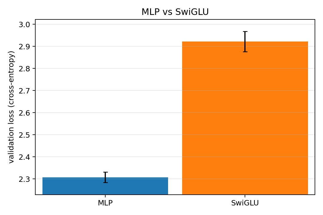
For the MLP vs SwiGLU comparison the result is a bit more surprising with the standard MLP handily beating out the more modern SwiGLU block. Still, a multilayer perceptron is still the default solution for a very simple neural network and SwiGLU has not taken its place across the board. Hence it is perhaps reasonable that the MLP stays strong when we're not pushing the boundaries of LLMs.

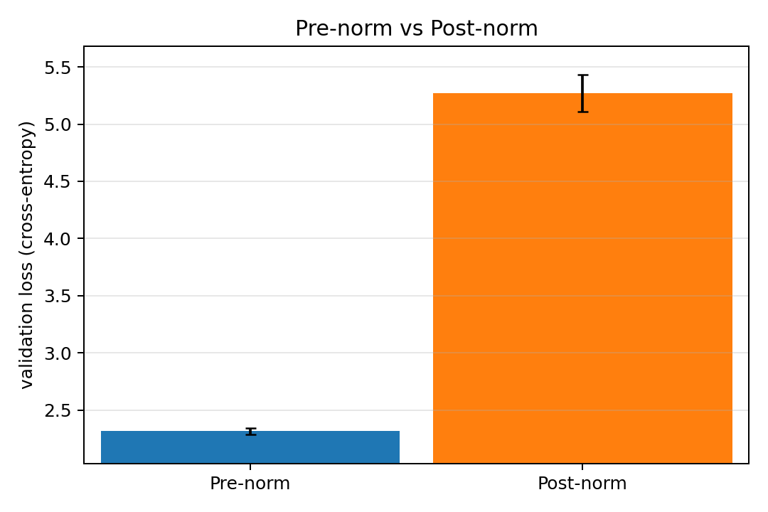
The difference between pre- and postnorm is absolutely huge in this case, enough so that I reran the experiment with a 30-minute training time (and reviewed the code) to be sure there was no issue with the implementation. At the longer training time, the gap persisted as pre-norm validation loss shrank to about 1.7 while post-norm remained at the same level. A likely explanation for the large discrepancy is that the learning rate was chosen too high to play well with post-norm as pre-norm improves training stability and the learning rate was chosen with pre-norm in mind. To test this out, I quickly tried at learning rate of 5e-4 which resulted in a significantly lower discrepancy but still a small edge for pre-norm. It is very possible that our decision to use mixed precision further increased the training instability problems for this high learning rate.

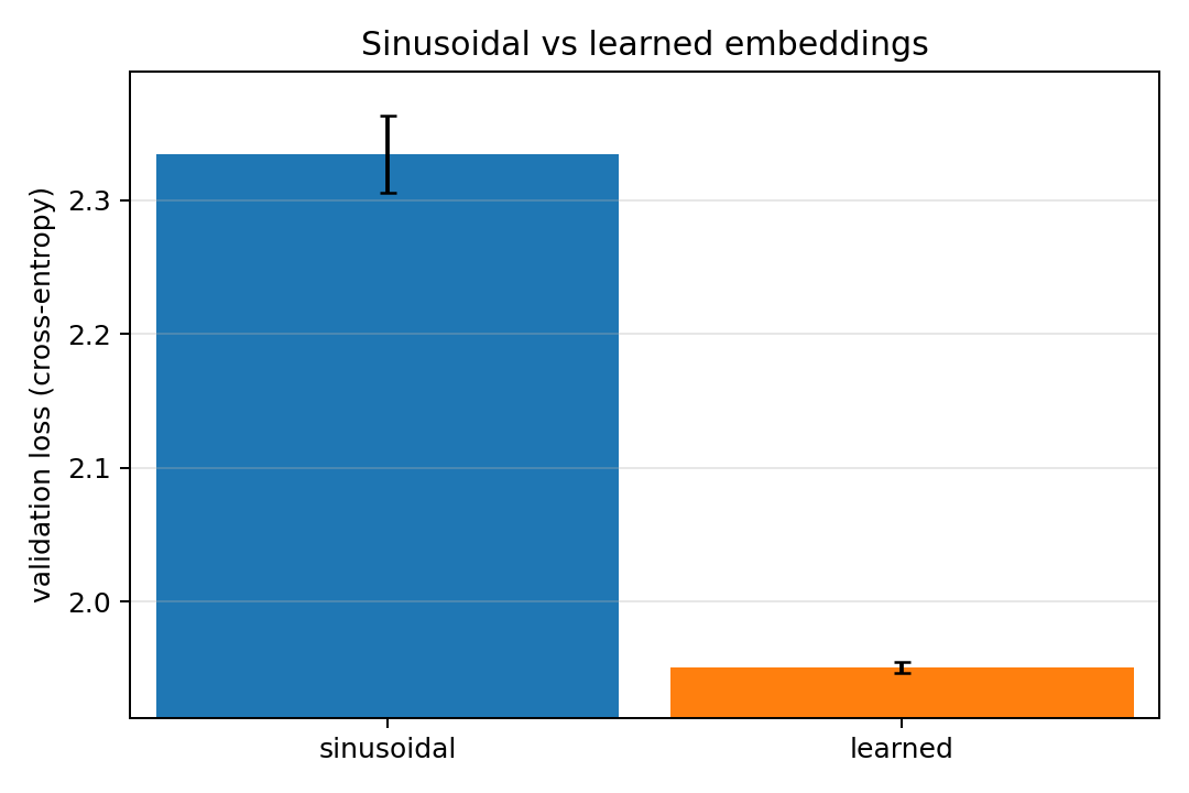
For the positional embeddings, learned embeddings turn out to perform better than sinusoidal ones. Perhaps because simpler embedding maps can co-evolve with the training instead of starting immediately with effectively 256 orthogonal embeddings to learn. In the early stages of training, simpler shorter relations for e.g., grammar are more important than longer dependencies which enable more coherence.

At this point, we should note that, with the exception of learned positional embeddings and a small change in the sizing, the choices in the original configuration were mostly correct. Before continuing with the dropout and gradient clipping sweeps, we take another look at learning rate and the optimizer for our updated configuration with learned positional embeddings. This also lets us choose a learning rate which is possibly better suited for the new choice of layers, heads and hidden dimension. We can also restrict our search to a tighter interval based on the earlier findings. Doing so we obtain the following results:

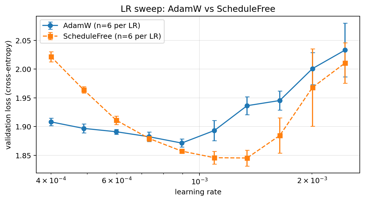
Based on this result, we switch the learning rate to 1.1e-3 and start using the Schedule-Free optimizer. We are now ready to continue with the dropout and gradient clipping sweeps.

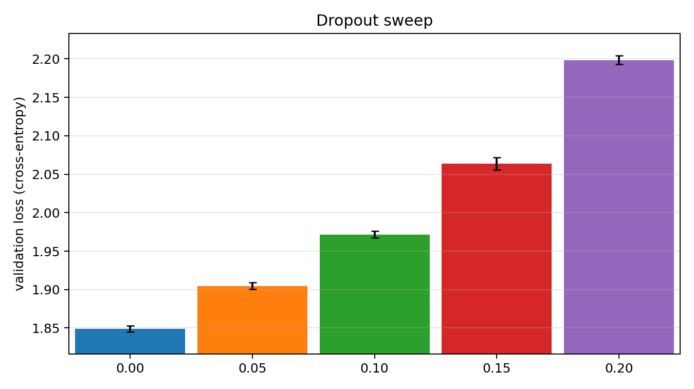
We see very clearly that dropout does not help which perhaps should be expected since we're training for around 1.7 epochs.

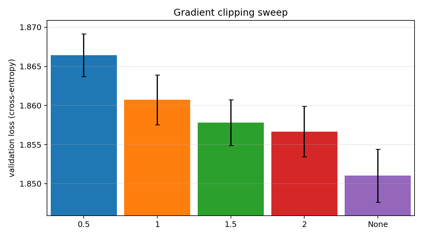
Lastly for the gradient clipping it certainly does not make a big difference and we keep it off.

Conclusions

The final model we end up with has 27.4M parameters and trains for around 30M tokens in the five minutes we give it to a validation loss of around 1.85 corresponding to a perplexity of 6.36. Many of the choices in the initial model configuration turned out to be correct which perhaps should be expected as they are standard choices for a reason. Still, at least for me, this investigation has highlighted how time intensive these sort of hyperparameter searches are and how many iterations it can take to reach a statistically significant answer.