Overview of masked spectrogram autoencoders for efficient pretraining
Vision transformers (ViTs) have since their introduction in 2020 become the de facto standard tool for computer vision tasks. While they are both highly performant in general and scale well with increased parameters, just as their NLP counterparts, they require large amounts of data to train. To tackle this problem, the team at FAIR released the paper Masked Autoencoders Are Scalable Vision Learners which proposed pretraining vision transformers with the self-supervised task of masked autoencoding - essentially infilling images. This was used to achieve state-of-the-art performance on ImageNet-1K without external data. We will discuss the main ideas in this paper as well as how the ideas have been adapted for audio tasks using spectrograms by building a simple implementation step-by-step.
The first usage of vision transformer for spectrograms was the Audio Spectrogram Transformer (AST) which pretrained on ImageNet to achieve state-of-the-art performance on a series of audio classification tasks after fine-tuning. The architecture of that model is essentially a standard vision transformer from the original paper An Image is Worth 16x16 Words: Transformers for Image Recognition at Scale, which at the time had been out for less than a year, applied to log-mel spectrograms of audio signals. More specialized models with stronger time-frequency inductive biases are not necessarily as easy to pretrain on image data and as such would require another approach.
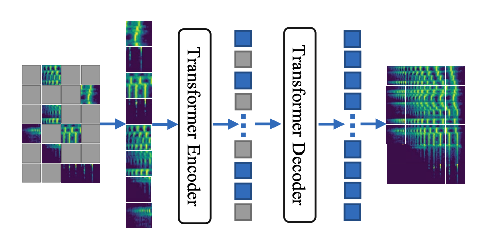
Masked autoencoding is essentially the (self-supervised) task of filling in the blanks of an image. As hinted at in the figure, the non-discarded patches of an image is passed to an encoder after which (learned) tokens corresponding to blank patches are inserted in the correct places and a decoder attempts to reconstruct the image. The network is trained by minimizing the mean squared error (MSE) on the patches initially blanked out. Before moving to implementing this and discussing the details of what changes need to be made for spectrograms, we discuss the basics of vision transformer to lay the groundwork.
Organization: We first go over the basics of vision transformers, then detail an implementation of masked autoencoders and finally present the results of applying it to spectrograms.
Basics of vision transformers
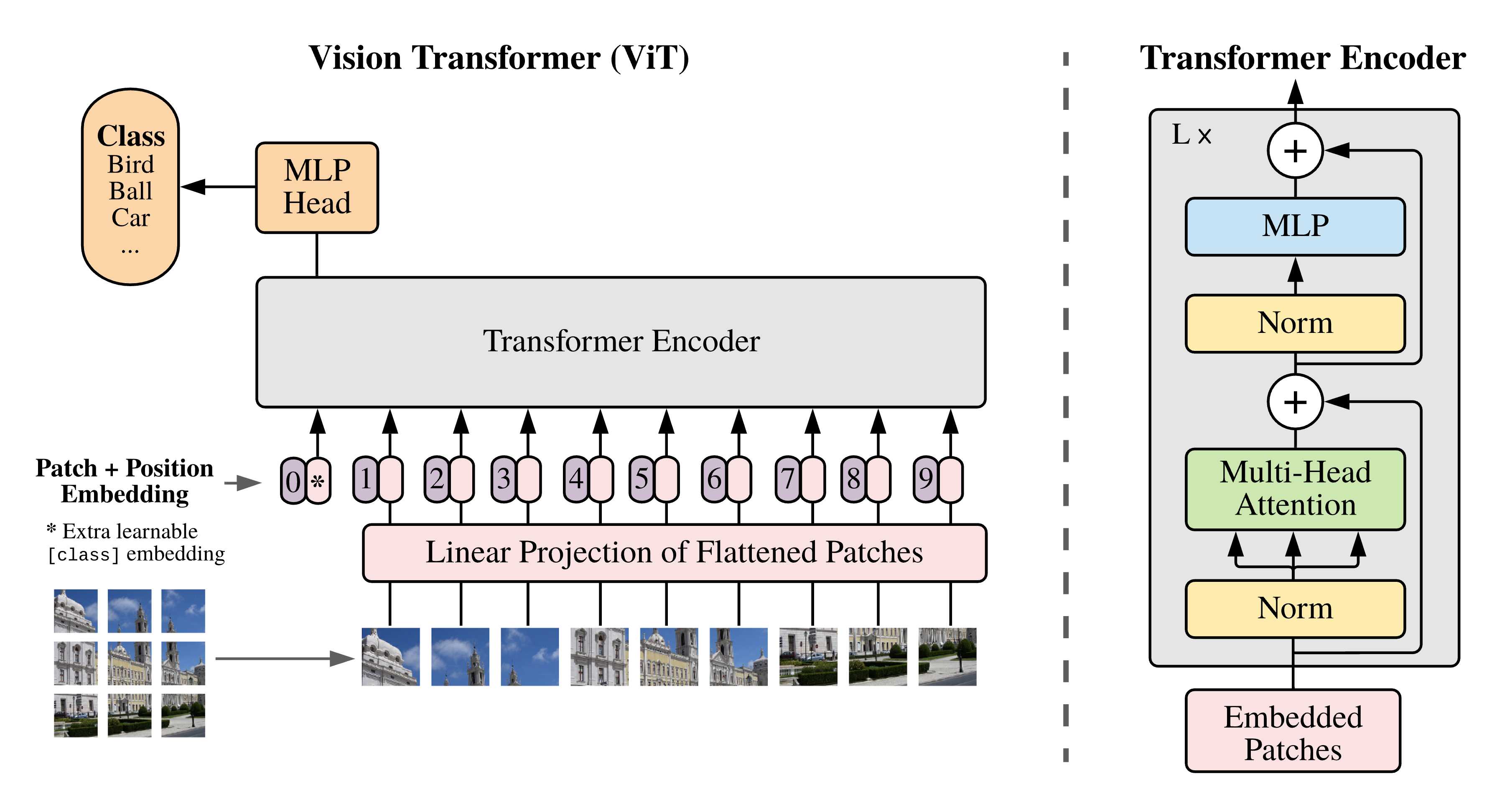
Any data which can be mapped to a series of high dimensional tokens can be acted on by a series of transformer blocks. Instead of these tokens representing words or parts of words as in the NLP context, vision transformers split an image up into smaller patches which are each mapped to d_model dimensional vectors by a linear projection. From there, the remainder of the transformer architecture is essentially unchanged. Later developments have added various features such as local attention (Swin Transformer) and translation-invariant convolution features (Convolutional vision Transformer) but we will stay away from these variants in the interest of simplicity.
The patching and subsequent linear projection of an image into d_model dimensional space is most efficiently implemented as a convolution with stride equal to the kernel width. If the original image is 224×224 and we want patches of size 14×14, we get 16×16 patches since 14×16=224. This procedure is implemented in the following way.
class PatchEmbedding(nn.Module):
	def __init__(self, patch_size, embed_dim):
		super(PatchEmbedding, self).__init__()
		self.conv = nn.Conv2d(1, embed_dim, kernel_size=patch_size, stride=patch_size)

	def forward(self, x):
		x = self.conv(x)

		x = x.flatten(2)
		x = x.transpose(1, 2)

		return x
Flattening and transposing makes it so our output tensor is of shape [batch_size, num_patches, embed_dim] which is what we want when this is passed to transformer blocks. The original ViT paper uses learned positional embeddings which for us is just a [16×16, d_model] tensor which we add onto the flattened patches. A good intuition behind why this is preferable to sinusoidal positional encodings is that some of the image topology can be encoded this way. After the positional embeddings, we prepend a learned [cls] token and put the resulting tensor through a series of encoder transformer blocks with full self-attention. Lastly the state of the [cls] token is passed through a MLP for classification via a vector of dimension num_classes.
class ViT(nn.Module):
	def __init__(
		self,
		width,
		height,
		num_classes,
		input_channels,
		patch_size,
		d_model,
		num_heads,
		num_layers,
		dropout,
	):
		super().__init__()
		self.d_model = d_model

		num_patches = (width // patch_size) * (height // patch_size)
		self.num_tokens = num_patches + 1
		self.patch_emb = PatchEmbedding(
			patch_size=patch_size, input_channels=input_channels, embed_dim=d_model
		)

		self.transformer_layers = nn.ModuleList(
			[
				nn.TransformerEncoderLayer(
					d_model,
					num_heads,
					dim_feedforward=d_model * 4,
					dropout=dropout,
					batch_first=True,
				)
				for _ in range(num_layers)
			]
		)

		self.cls_token = nn.Parameter(torch.randn(1, 1, self.d_model))
		self.pos_emb = nn.Parameter(torch.randn(1, self.num_tokens, self.d_model))

		self.final_mlp = nn.Linear(self.d_model, num_classes)

	def forward(self, x):
		batch_size = x.size(0)

		x = self.patch_emb(x)
		cls_token = self.cls_token.expand(batch_size, 1, self.d_model)

		x = torch.cat((cls_token, x), dim=1)
		x = x + self.pos_emb.expand(batch_size, self.num_tokens, self.d_model)

		for layer in self.transformer_layers:
			x = layer(x)

		x = self.final_mlp(x[:, 0, :])

		return x
The model is now ready to be trained. With the Tiny ImageNet dataset consisting of 100,000 RGB images with resolution 64×64, grouped into 200 classes, we can set up the following PyTorch Dataset:
class TinyImageNetDataset(Dataset):
	def __init__(self, dataset_split, transform=None):
		self.dataset = dataset_split
		self.transform = transform

	def __len__(self):
		return len(self.dataset)

	def __getitem__(self, idx):
		img = self.dataset[idx]['image']
		label = self.dataset[idx]['label']

		if self.transform:
			img = self.transform(img)

		return img, label
For the transforms, we use a custom class EnsureRGB which deals with black and white images by essentially only calling img.convert('RGB') on the PIL image, ToTensor which maps the PIL image to a tensor and Normalize with the mean and standard deviation from the full ImageNet. We could have normalized using mean = 0, std = 1 but the difference between channels is actual information which we have no reason to keep from the model.
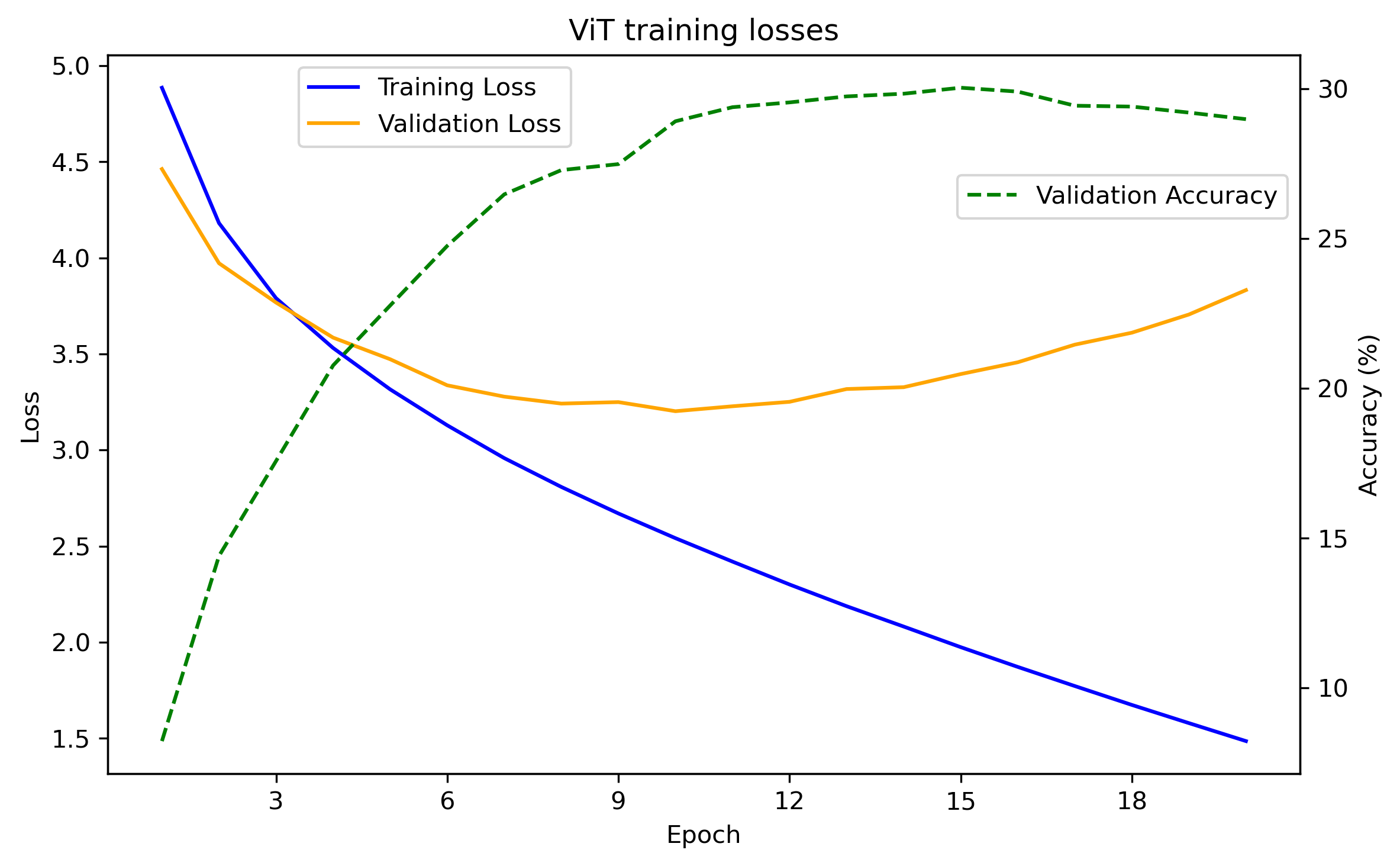
Training a standard training loop (see here for further details) with patch_size = 8, d_model = 256, num_heads = 4, num_layers = 4, dropout = 0.1 we get the following losses and accuracies:
We see that we get into overfitting territories after about 10 epochs and that the accuracy peaks at around 30% over the 200 classes.
Remark: This is a fairly weak result. State of the art for Tiny ImageNet is above 90% and obviously benefits from extensive pretraining. However training a ResNet-18 model from scratch with the same setup results in an accuracy of ~32% so it is not the inherent drawbacks of vision transformers that we are limited by.
Masked autoencoders
We will build a model which can be toggled between masked autoencoder mode and vision transformer mode which we will pretrain with model.mode == 'mae' and finetune with model.mode == 'vit'.
The encoder part of our masked autoencoder is for the most part the same as the vision transformer without the final MLP classification head. The crucial difference is that it should be able to act on a subset of all possible tokens. We use the same PatchEmbedding class to encode the image into a sequence of tokens and add positional encodings to all patches. For simplicity, we drop the [CLS] token and will instead use average pooling over the tokens as the input for our final classifier. Before acting on the tokens by the transform blocks, we randomly drop mask_ratio×num_tokens patches using the following function.
def remove_tokens(x, mask):
	batch_size, tokens, d_model = x.size()
	kept_tokens = math.ceil(tokens * mask)

	mask_indices = torch.zeros(batch_size, tokens, dtype=torch.bool, device=x.device)

	for i in range(batch_size):
		perm = torch.randperm(tokens, device=x.device)
		selected = perm[:kept_tokens]
		mask_indices[i, selected] = True

	mask_expanded = mask_indices.unsqueeze(-1).expand(-1, -1, d_model)
	shortened_tensor = x[mask_expanded].view(batch_size, kept_tokens, d_model)

	return shortened_tensor, mask_indices
Note that the mask_indices tensor is returned from this function. Without the __init__() method, the first part of our models forward() function will then look as follows.
def forward(self, x):
	batch_size = x.size(0)

	x = self.patch_emb(x)
	x = x + self.pos_emb_enc.expand(batch_size, self.num_patches, self.d_model)

	if self.mode == 'mae':
		x, mask_indices = remove_tokens(x, self.mask_ratio)

	for layer in self.transformer_encoder_layers:
		x = layer(x)

	encoded = x

	if self.mode == 'vit':
		x = torch.mean(x, dim=1)
		x = self.classification_mlp(x)
		return x

	...
The encoded state will be passed to the transformer decoder blocks for cross-attention. Before passing x onto these blocks, we need to make it consist of num_tokens again by infilling the locations where tokens were removed. We do this using learned default tokens for each location.
def infill_tokens(shortened_tensor, default_tensor, mask_indices):
	batch_size = default_tensor.size(0)
	reconstructed_tensor = default_tensor.clone()

	for i in range(batch_size):
		reconstructed_tensor[i][mask_indices[i]] = shortened_tensor[i]

	return reconstructed_tensor
After infilling and adding positional embeddings, the core of the decoder is a series of decoder transformer blocks with cross-attention with the encoded state. To return to an image, we map each token to a patch with a nn.Linear(d_model, patch_size**2 * channels) and reshape to be of shape [channels, width, height].
    def forward(self, x):
        ...

        default_tokens = self.default_tokens.expand(batch_size, self.num_patches, self.d_model)
        x = infill_tokens(x, default_tokens, mask_indices)

        x = x + self.pos_emb_dec.expand(batch_size, self.num_patches, self.d_model)

        for layer in self.transformer_decoder_layers:
            x = layer(tgt = x, memory = encoded)

        x = self.patchify_mlp(x)
        x = self.reverse_patch_embedding(x)

        return x
The function reverse_patch_embedding maps tensors from shape [batch_size, num_patches, patch_size**2 * channels] to [batch_size, channels, width, height].
def reverse_patch_embedding(self, x):
	batch_size = x.size(0)
	tokens = x.size(1)
	H_p = self.height // self.patch_size
	W_p = self.width // self.patch_size

	x = x.view(batch_size, H_p, W_p, self.channels, self.patch_size, self.patch_size)
	x = x.permute(0, 3, 1, 4, 2, 5).contiguous()
	x = x.view(batch_size, self.channels, H_p * self.patch_size, W_p * self.patch_size)

	return x
class MAE(nn.Module):
	def __init__(
		self,
		width,
		height,
		num_classes,
		channels,
		patch_size,
		enc_num_heads,
		enc_num_layers,
		dec_num_heads,
		dec_num_layers,
		d_model,
		dropout,
		mask_ratio
	):
		super().__init__()
		self.d_model = d_model

		self.channels = channels
		self.width = width
		self.height = height
		self.patch_size = patch_size
		self.channels = channels
		self.num_patches = (width // patch_size) * (height // patch_size)
		self.patch_emb = PatchEmbedding(
			patch_size=patch_size, input_channels=channels, embed_dim=d_model
		)
		self.mask_ratio = mask_ratio
		self.mode = 'vit' if mask_ratio == 0.0 else 'mae'

		self.transformer_encoder_layers = nn.ModuleList(
			[
				nn.TransformerEncoderLayer(
					d_model,
					enc_num_heads,
					dim_feedforward=d_model * 4,
					dropout=dropout,
					batch_first=True,
				)
				for _ in range(enc_num_layers)
			]
		)

		self.transformer_decoder_layers = nn.ModuleList(
			[
				nn.TransformerDecoderLayer(
					d_model,
					dec_num_heads,
					dim_feedforward=d_model * 4,
					dropout=dropout,
					batch_first=True,
				)
				for _ in range(dec_num_layers)
			]
		)

		self.pos_emb_enc = nn.Parameter(torch.randn(1, self.num_patches, self.d_model))
		self.pos_emb_dec = nn.Parameter(torch.randn(1, self.num_patches, self.d_model))
		self.default_tokens = nn.Parameter(torch.rand(1, self.num_patches, self.d_model))

		self.classification_mlp = nn.Linear(self.d_model, num_classes)
		self.patchify_mlp = nn.Linear(self.d_model, self.patch_size**2 * self.channels)

	def reverse_patch_embedding(self, x):
		batch_size = x.size(0)
		tokens = x.size(1)
		H_p = self.height // self.patch_size
		W_p = self.width // self.patch_size

		x = x.view(batch_size, H_p, W_p, self.channels, self.patch_size, self.patch_size)
		x = x.permute(0, 3, 1, 4, 2, 5).contiguous()
		x = x.view(batch_size, self.channels, H_p * self.patch_size, W_p * self.patch_size)

		return x

	def forward(self, x):
		batch_size = x.size(0)

		x = self.patch_emb(x)
		x = x + self.pos_emb_enc.expand(batch_size, self.num_patches, self.d_model)

		if self.mode == 'mae':
			x, mask_indices = remove_tokens(x, self.mask_ratio)

		for layer in self.transformer_encoder_layers:
			x = layer(x)

		encoded = x

		if self.mode == 'vit':
			x = torch.mean(x, dim=1)
			x = self.classification_mlp(x)
			return x

		default_tokens = self.default_tokens.expand(batch_size, self.num_patches, self.d_model)
		x = infill_tokens(x, default_tokens, mask_indices)

		x = x + self.pos_emb_dec.expand(batch_size, self.num_patches, self.d_model)

		for layer in self.transformer_decoder_layers:
			x = layer(tgt = x, memory = encoded)

		x = self.patchify_mlp(x)
		x = self.reverse_patch_embedding(x)

		return x
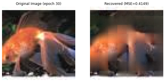
If we now run the model with mask_ratio > 0 we get a working infilling model. This training target is very complex and for great results require some form of world model, a part of which is understanding what sort of object is pictured. Consequently the reconstruction loss keeps decreasing over many epochs and we get the following results with mask_ratio = 0.75 which is reported as optimal in the ImageNet-1K case in the original paper.
The above example is only illustrative and by pretraining on larger datasets much more convincing reconstructions can be obtained. Instead of focusing on that, we switch our focus to spectrograms where we will pretrain and finetune our model.
Application to spectrograms
The paradigm of applying computer vision methods to spectrogram or similar data for signal processing tasks such as classification, automatic speech recognition (ASR) and music information retrieval (MIR) has a long history and versions of it are used in state of the art systems. While earlier models relied on convolutional neural networks (CNNs), newer methods such as the Audio Spectrogram Transformer (AST) use a ViT backbone. Contemporary state of the art ASR methods such as Whisper and Conformer tokenize along the time dimension instead of evenly spaced patches in time and frequency but the underlying architecture is still similar.
We will train a ViT for audio classification on the Speech Commands V2 dataset by first pretraining a masked autoencoder task on 360 hours of LibriSpeech and compare with no pretraining. This is very similar to what was done in Masked Spectrogram Prediction For Self-Supervised Audio Pre-Training mentioned earlier, where pretraining was done on AudioSet and evaluated on a collection of downstream tasks. Meanwhile it differs from the pretraining setup in AST where the pretraining on AudioSet only used a classification task.
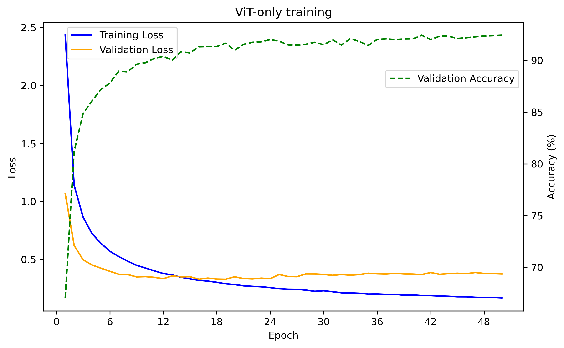
The input spectrograms we will use are log-mel spectrograms with 128 mel filters and n_fft = 1024 which corresponds to around 64 ms time windows, resulting in 1s spectrograms of resolution 64×128. Our ViT encoder uses a slightly scaled down version of ViT-B with d_model = 512, num_layers = 8 and num_heads = 8 and 16×16 patches. With no pretraining and a basic data augmentation setup consisting of white noise, spectrogram blurring and time/frequency masking, we get a 91.89% test accuracy with the following train/validation curves.
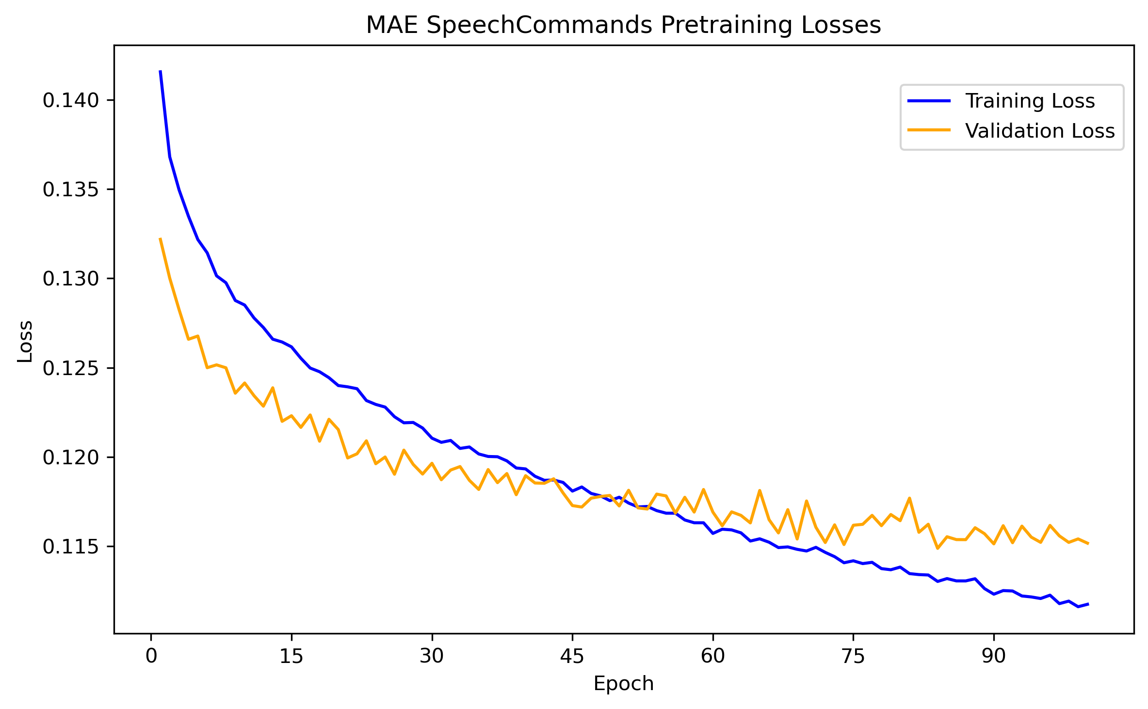
With this as our baseline we now move to the masked autoencoder version. As earlier, programmatically the masked autoencoder is the same model with model.mode = 'mae'. LibriSpeech works great for the initial pretraining as its contents is people talking and the recording environment is not too dissimilar to that of SpeechCommands V2. For each audioclip, we take a random 1 second snippet and train for 100 epochs. After this, we do the same pretraining on SpeechCommands V2 for another 100 epochs. The train/validation losses keep decreasing throughout but clearly we are getting into overfitting territory as can be seen in the figure.
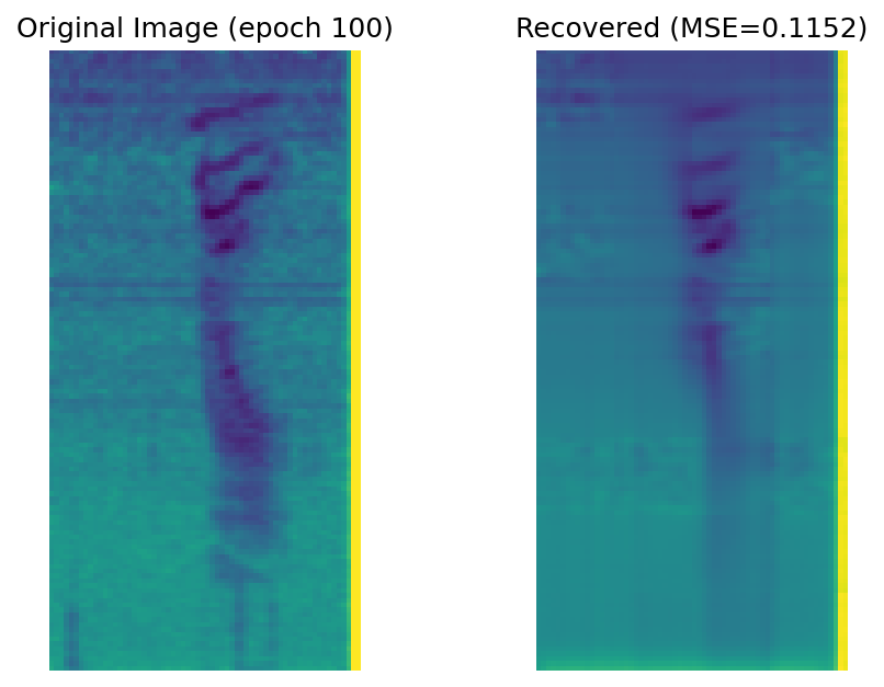
With 75% of the spectrogram masked, the reconstructed spectrograms are far from perfect and reconstructing the noise of masked patches is obviously impossible.
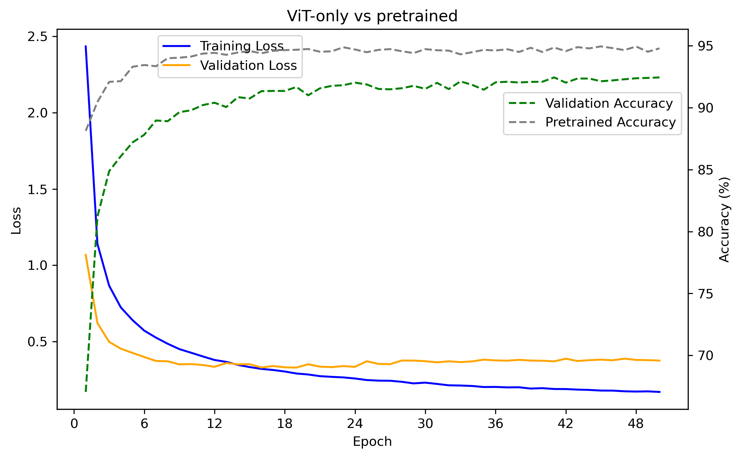
After the pretraining we set the model in ViT mode and train on SpeechCommands V2 classification again with significantly improved results.
The test accuracy for the checkpoint with the highest validation accuracy is 94.63% meaning that pretraining improved the classification result by about 3 percentage points.
