On the role of phase in ML audio noise reduction
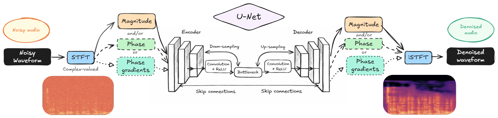
A standard way of reducing the noise of audio or another signal with some form of time-frequency structure using a machine learning approach is as follows: Compute the short-time Fourier transform of the signal, map it to a "clean" spectrogram using a U-Net, and then synthesize a signal back. In the simplest version of this construction, the U-Net returns a real-valued mask over the time-frequency plane, telling us which time-frequency bins to ignore in the reconstruction and which to keep. This approach reuses the noisy phase values of the original signal.
In this post we look at more intricate versions of this construction that go beyond time-frequency multipliers by paying more attention to the phase of the output. The idea is to highlight the concepts behind these versions and indicate how they are encoded in PyTorch.
After covering some background and context, we will discuss three STFT U-Net based noise reduction methods which all utilize phase in different ways. The goal is not to determine which one is optimal, that is dependent on the specific task, but rather to show that all three work and discuss their respective strengths.
Background
To keep the post focused, we will assume the reader has a basic familiarity with the short-time Fourier transform (STFT) and spectrograms as 2D representations of signals which allows simultaneous inspection of the time and frequency contents. A key fact about the STFT is that any signal (vector) has a STFT (2D matrix) but not all 2D matrices (of the correct shape) correspond to a signal. This can be seen as a consequence of the uncertainty principle which puts limits on the time-frequency localization of a signal.
Phase in the STFT
Since the STFT is complex-valued, it is often visualized via its absolute values, the spectrogram. The role of the phase of the STFT was not clear in the early days of time-frequency analysis. Indeed, energy is a much more familiar concept and that is determined only by the absolute value of the STFT. Moreover, as phase retrieval has shown, knowing the spectrogram the phase can be recovered up to a global unimodular factor.
So what happens if we have a 2D matrix of the correct shape of complex numbers and want to synthesize a signal from it but the phase and/or magnitude are not chosen so that they correspond to an actual signal? Such a matrix is said to be inconsistent but if we still do synthesize a signal by means of the inverse STFT, we do get a signal. What happens is that we implicitly compute the orthogonal projection onto the subspace of consistent matrices, the Gabor projection. This is fine, after all orthogonal projections are the best kind, but the resulting audio signal may sound a little weird to human ears.
The best way to illustrate this is by an example. A pure sine tone has a sharp frequency concentration and a predictable STFT phase behavior, the phase changes evenly over time.
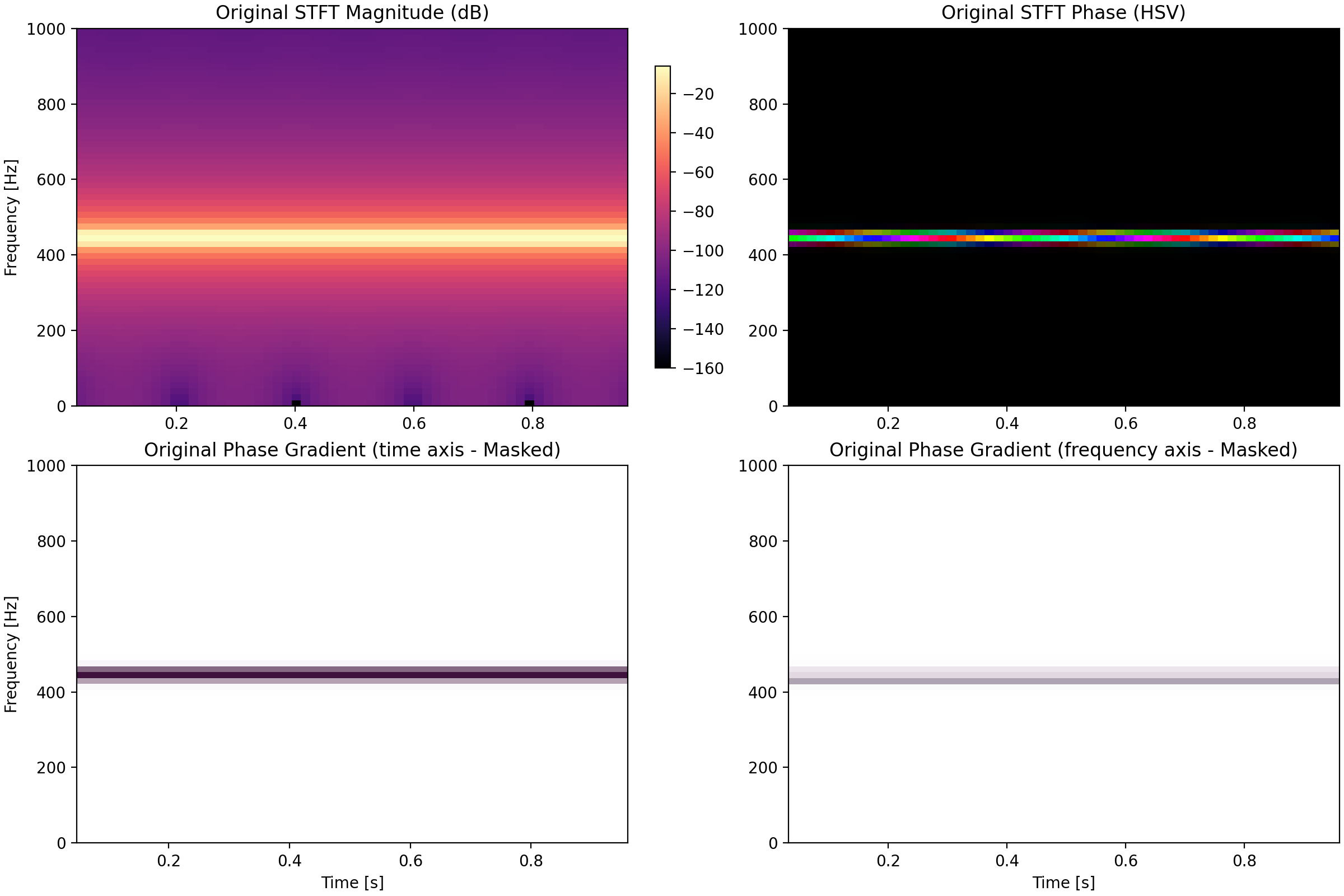
If we take this STFT and randomize the phase and synthesize a signal back, we get a much less nicely structured STFT from the resulting waveform.
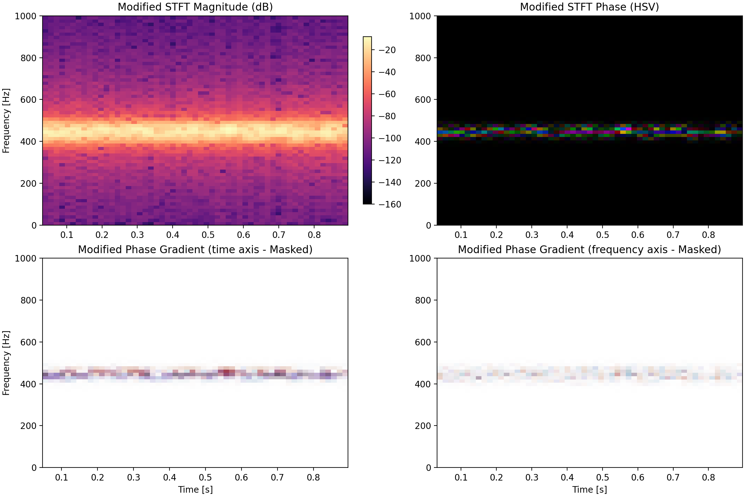
Here we see that the Gabor projection has changed the magnitude of the STFT as well, even though it is only the phases we changed. The phase gradients are a lot less even which is the main takeaway. The change can be heard in the following comparison.
Listening to these examples, we hear the same tone but with a weird form of non-pureness in the modified version. It is this type of phase-induced error which we are looking to avoid in this post.
U-Nets
We are looking to modify the STFT of our input signal. Forgetting about modern diffusion-based image-to-image models for a while, the standard way to do this is via a U-Net.
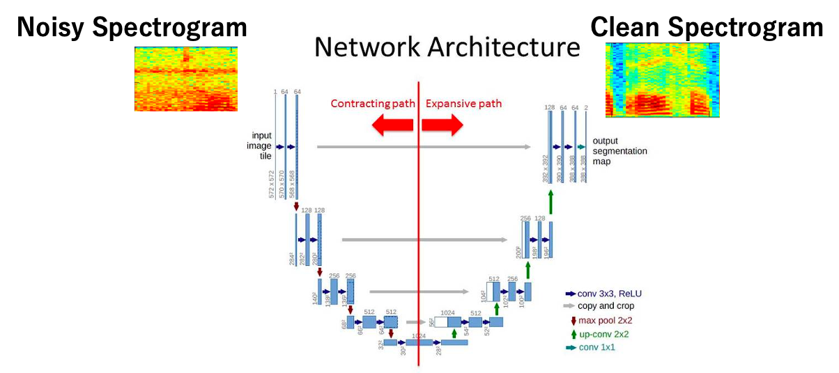
This architecture is more than 10 years old and should be considered a commodity by now. We reproduce the version used here below for reference.
class ConvBlock(torch.nn.Module):
    def __init__(self, in_channels, out_channels):
        super().__init__()
        self.net = torch.nn.Sequential(
            torch.nn.Conv2d(in_channels, out_channels, kernel_size=3, padding=1),
            torch.nn.ReLU(inplace=True),
            torch.nn.Conv2d(out_channels, out_channels, kernel_size=3, padding=1),
            torch.nn.ReLU(inplace=True),
        )

    def forward(self, x):
        return self.net(x)


class UNet2D(torch.nn.Module):
    def __init__(self, in_channels=1, base_channels=16, out_channels=1, use_sigmoid=True):
        super().__init__()
        self.enc1 = ConvBlock(in_channels, base_channels)
        self.enc2 = ConvBlock(base_channels, base_channels * 2)
        self.enc3 = ConvBlock(base_channels * 2, base_channels * 4)
        self.enc4 = ConvBlock(base_channels * 4, base_channels * 8)
        self.bottleneck = ConvBlock(base_channels * 8, base_channels * 16)

        self.pool = torch.nn.MaxPool2d(2)

        self.dec4 = ConvBlock(base_channels * 16 + base_channels * 8, base_channels * 8)
        self.dec3 = ConvBlock(base_channels * 8 + base_channels * 4, base_channels * 4)
        self.dec2 = ConvBlock(base_channels * 4 + base_channels * 2, base_channels * 2)
        self.dec1 = ConvBlock(base_channels * 2 + base_channels, base_channels)

        self.out_conv = torch.nn.Conv2d(base_channels, out_channels, kernel_size=1)
        self.use_sigmoid = use_sigmoid

    def _upsample_to(self, x, target):
        return F.interpolate(x, size=target.shape[-2:], mode="nearest")

    def forward(self, x):
        e1 = self.enc1(x)
        e2 = self.enc2(self.pool(e1))
        e3 = self.enc3(self.pool(e2))
        e4 = self.enc4(self.pool(e3))
        b = self.bottleneck(self.pool(e4))

        d4 = self._upsample_to(b, e4)
        d4 = self.dec4(torch.cat([d4, e4], dim=1))

        d3 = self._upsample_to(d4, e3)
        d3 = self.dec3(torch.cat([d3, e3], dim=1))

        d2 = self._upsample_to(d3, e2)
        d2 = self.dec2(torch.cat([d2, e2], dim=1))

        d1 = self._upsample_to(d2, e1)
        d1 = self.dec1(torch.cat([d1, e1], dim=1))

        output = self.out_conv(d1)
        if self.use_sigmoid:
            output = torch.sigmoid(output)
        return output
Dataset
Since our focus is more on the method than the data and performance, we take a simple approach to the data. Specifically, we use the Common Voice Scripted Speech 24.0 - Swedish subset which is 1.13 GB. This dataset is not perfectly noise-free nor is it incredibly large but it is easily accessible and generally of high quality. To create noisy data, we add white noise to the waveform with energy between 0% and 60% of that of the waveform, then normalize the noisy version to have energy 1 and use the same scale factor for the clean version so that the target has less energy but the network does not know a priori how much energy it is supposed to have.
We could also have added different sorts of noise $\mathcal{N}$ (pink noise, environmental noise, etc.) to make the algorithm more robust but we skip this in the interest of simplicity.
Take 1: Time-frequency multiplier
If we want to attack noise reduction using machine learning we need to identify the loss function we wish to train using. While mean squared error (MSE) is a tried and true method, it has a clear disadvantage when it comes to audio tasks: The human ear does not hear (waveform) phase. For example, we cannot distinguish between $f$ and $-f$, yet $\operatorname{MSE}(f, -f) > 0$. There is a classical blog post by Evan Radkoff on loss functions in Audio ML with many details and suggestions but we will settle with just looking at the spectrogram $L^1$ distance, defined as $\Vert \operatorname{SPEC}(f) - \operatorname{SPEC}(g) \Vert_{L^1}$. This loss function is phase invariant and easy to understand; we want to match the time-frequency distribution of the energy.
Now in this simplest version of noise reduction, the U-Net will only act to modify the magnitudes of the STFT and only take the magnitudes as input data to the U-Net. This means that, with $V_g f$ the STFT and $V_g f^*$ the inverse STFT, the pipeline can be written as
where $A_g^m$ is a so-called Gabor multiplier with mask $m$. While Gabor multipliers are nicely behaved linear maps, U-Nets very much are not, which is the whole point.
Programmatically, we can write this model as follows:
class SpectrogramMaskUNet(torch.nn.Module):
    def __init__(self):
        super().__init__()
        self.n_fft = N_FFT
        self.unet = UNet2D(in_channels=1, base_channels=16)
        self.register_buffer("window", torch.hann_window(WINDOW_LENGTH))

    def forward(self, waveform):
        stft = torch.stft(
            waveform.squeeze(1),
            n_fft=N_FFT,
            hop_length=HOP_LENGTH,
            win_length=WINDOW_LENGTH,
            window=self.window,
            return_complex=True,
        )
        mag = stft.abs()
        mag_in = mag.unsqueeze(1)
        mask = self.unet(mag_in)
        masked_stft = stft * mask.squeeze(1)

        denoised = torch.istft(
            masked_stft,
            n_fft=N_FFT,
            hop_length=HOP_LENGTH,
            win_length=WINDOW_LENGTH,
            window=self.window,
            length=waveform.shape[-1],
        )

        return denoised.unsqueeze(1), mask
Training for a few epochs, we get acceptable performance such as in the following example.
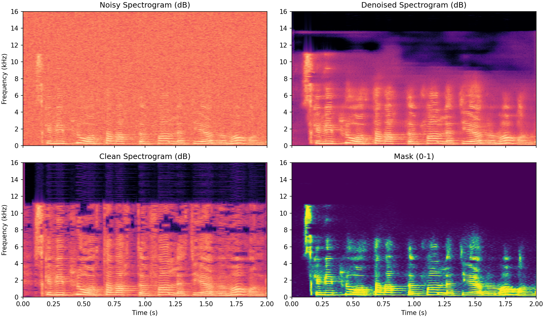
Here the mask itself almost looks like a spectrogram because it has identified the specific parts where the actual audio is coming in. The clean spectrogram is also not entirely noise free in this example which most likely is limiting the learning potential of the network. Still, the general principle of there being many ways to be wrong but only one to be right applies here and the denoised version appears to have gotten rid of at least some of the higher frequency artifacts of the clean version.
The audio for this particular example can be played here.
Note that since we have not changed the phase of the noisy spectrogram, we are subject to the noisy phase messing up the resulting signal in the same way as we illustrated earlier. This is a clear limitation but in return we get a method which is very structured. By forcing the output to use the phase data from the original noisy output and capping the mask at $1$ we place limits on how much we can diverge from the original (noisy) input signal. This can be valuable due to the high explainability of this method. In this next method, we trade some of this explainability for expressiveness.
Take 2: 2-channel complex STFT prediction
One way to lift the limitations just discussed with the masking approach is to give up the multiplicative formulation. Specifically, we can let a U-Net map the noisy STFT to a 2D matrix of complex numbers of the same shape and then synthesize a signal from that. By doing so, we move away from the time-frequency structured approach of the earlier method and take a step towards an end-to-end solution.
With this approach, we are letting the phases into the U-Net directly. There are a few different ways to go about this. Perhaps the simplest one is to let the U-Net map to and from an image with 2 channels (real + imaginary, or magnitude + phase). Predicting phase in $[-\pi, \pi]$ is difficult due to the wrapping behavior so we go with the continuous approach of predicting real and imaginary values as two channels.
The only modifications needed on the model side is to not apply sigmoid activation to the last layer of the U-Net and to encode/decode complex numbers in two channels.
class Spectrogram2ChannelUNet(torch.nn.Module):
    def __init__(self):
        super().__init__()
        self.n_fft = N_FFT
        self.unet = UNet2D(
            in_channels=2,
            base_channels=16,
            out_channels=2,
            use_sigmoid=False,
        )
        self.register_buffer("window", torch.hann_window(WINDOW_LENGTH))

    def forward(self, waveform):
        stft = torch.stft(
            waveform.squeeze(1),
            n_fft=N_FFT,
            hop_length=HOP_LENGTH,
            win_length=WINDOW_LENGTH,
            window=self.window,
            return_complex=True,
        )
        stft_in = torch.stack([stft.real, stft.imag], dim=1)
        stft_out = self.unet(stft_in)
        out_complex = torch.complex(stft_out[:, 0], stft_out[:, 1])

        denoised = torch.istft(
            out_complex,
            n_fft=N_FFT,
            hop_length=HOP_LENGTH,
            win_length=WINDOW_LENGTH,
            window=self.window,
            length=waveform.shape[-1],
        )

        return denoised.unsqueeze(1), out_complex
Training this model for a few epochs, we get results of the following sort.
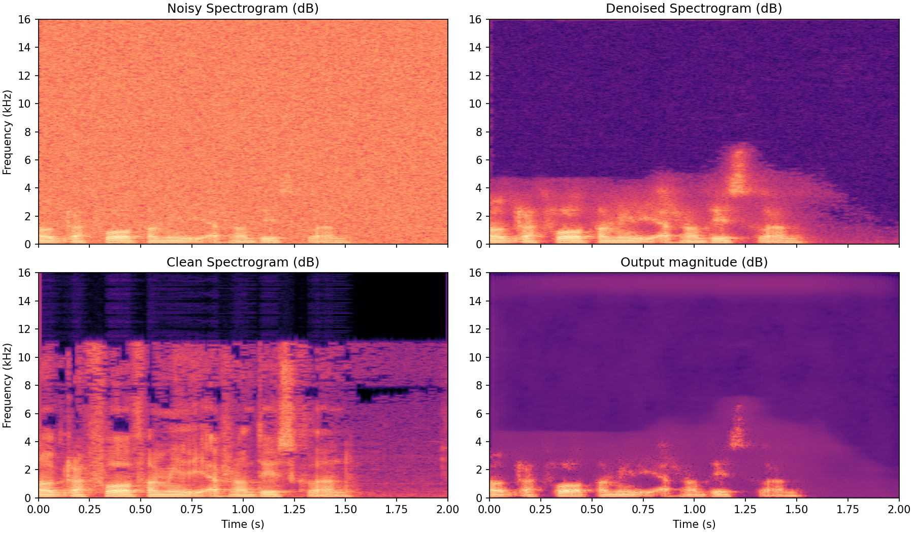
Compared to the mask approach, this output is less bound to the structure of the input spectrogram and seemingly retains less of the noise of the clean signal. Training this model is a bit less predictable, more training runs ended up in local minima. While this should be easy to counteract (change optimizer, learning rate or scheduler) it should be seen as a consequence of this method being more end-to-end.
The main weakness of this approach is what we will attempt to remedy in the final method; the loss is invariant to a global change of phase so the model will struggle to learn how to choose the output phase.
Take 3: STFT phase gradient prediction
The obvious way to solve the problem of the global phase invariance is to not output the phase, but instead the phase gradient $\nabla \Phi$. At this point, it is important to remark that the training target and the model output is liable to diverge. Indeed, going from the phase gradients to a consistent phase is non-trivial. It is very unlikely that we can find a function $\Phi$ with a prescribed $\nabla \Phi$ since it is a function on a 2D space. Instead we can try to solve this problem approximately, either via a phase integrator which attempts to find the phase at a prescribed point by integrating up to it, or by minimizing a functional of the form
where $F$ is the prescribed phase gradient. The phase integrator, while convoluted (there are many ways to integrate to each point) can be formulated in a differentiable way. The same can not be said for the general concept of minimizing the above functional. However, there is no inherent need for this final step to differentiable. During training we have access to the clean phase gradients which we can use for the loss function, and the process of actually determining the phase can happen outside the training process.
Gradient matching loss function
Outputting the gradients directly raises a new issue - what is the appropriate loss function? Let $\phi_x$ be the target derivative in the $x$ direction, $\hat{\phi}_x$ the network output and $\Delta_x =\phi_x - \hat{\phi}_x$. Then we want the loss to satisfy $L(\Delta) = L(\Delta + 2\pi)$. One way to solve this problem is to choose
which is connected to the von-Mises distribution. For small $\Delta$, this loss function is quadratic which is desirable. Another quadratic solution is to wrap $\Delta$ to $[-\pi, \pi]$ as
and choose $L(\Delta) = \operatorname{wrap}(\Delta)^2$. This sidesteps the problem of flatness of derivative of $1-\cos(\Delta)$ for $\Delta$ near $\pi$ at the cost of nondifferentiability at a point. A third way is to output two numbers $\hat{c}, \hat{s}$, choose $\hat{\phi}_x = \operatorname{atan2}(\hat{c}, \hat{s})$ and $ L = | \hat{c} + i\hat{s} - e^{i\phi_x} |$. All approaches are valid but in the interest of simplicity we will go with the squared wrapping option for our approach.
Note also that having the correct phase gradient is only important if the related time-frequency bin has energy. Therefore we will weigh the gradient loss function by the associated clean magnitude. After adding a loss term for the magnitude prediction as well, the total loss function becomes
The precise weighing of the amplitude (linear, quadratic, logarithmic) should be considered as a hyperparameter. The choices we have made here are not necessarily optimal. In PyTorch we can formulate this loss as follows:
class PhaseGradientLoss(torch.nn.Module):
    def __init__(self, n_fft=N_FFT, hop_length=HOP_LENGTH, win_length=WINDOW_LENGTH):
        super().__init__()
        self.n_fft = int(n_fft)
        self.hop_length = int(hop_length)
        self.win_length = int(win_length)
        self.register_buffer("window", torch.hann_window(self.win_length))

    def forward(self, clean, pred):
        clean_mono = clean.squeeze(1)
        stft = torch.stft(
            clean_mono,
            n_fft=self.n_fft,
            hop_length=self.hop_length,
            win_length=self.win_length,
            window=self.window,
            return_complex=True,
        )
        target_mag = stft.abs()
        target_phase = torch.angle(stft)
        target_phi_x, target_phi_y = compute_phase_gradients(target_phase)

        pred_mag = pred["mag"]
        pred_phi_x = pred["phi_x"]
        pred_phi_y = pred["phi_y"]

        mag_loss = F.mse_loss(pred_mag, target_mag)

        delta_x = wrap_phase(pred_phi_x - target_phi_x)
        delta_y = wrap_phase(pred_phi_y - target_phi_y)
        weight = target_mag
        grad_loss = (weight * (delta_x.abs()**2 + delta_y.abs()**2)).mean()

        return mag_loss + grad_loss
The function compute_phase_gradients() is a helper function that does precisely what you expect.
Implementation
For training the actual network, since we are outputting the final denoised spectrogram but rather a suggested amplitude and phase gradient which later on needs to be married, we let the U-Net map to and from the magnitude and phase gradients. However, a phase gradient of $\pi$ is equivalent to one of $-\pi$ so we want these points to be close together. Therefore, instead of passing phi_x and phi_y into the U-Net, we encode these angles by their location on the unit circle. That means we pass in $\cos(\phi_x), \sin(\phi_x)$, etc. and decode using atan2.
class SpectrogramPhaseGradientUNet(torch.nn.Module):
    def __init__(self):
        super().__init__()
        self.n_fft = N_FFT
        self.unet = UNet2D(
            in_channels=5,
            base_channels=32,
            out_channels=5,
            use_sigmoid=False,
        )
        self.register_buffer("window", torch.hann_window(WINDOW_LENGTH))

    def forward(self, waveform):
        stft = torch.stft(
            waveform.squeeze(1),
            n_fft=N_FFT,
            hop_length=HOP_LENGTH,
            win_length=WINDOW_LENGTH,
            window=self.window,
            return_complex=True,
        )
        mag_in = stft.abs()
        phase = torch.angle(stft)
        phi_x_in, phi_y_in = compute_phase_gradients(phase)
		#pass in phase gradients mapped to unit circle
        stft_in = torch.stack([mag_in,
                               torch.cos(phi_x_in),
                               torch.sin(phi_x_in),
                               torch.cos(phi_y_in),
                               torch.sin(phi_y_in)], dim=1)

        stft_out = self.unet(stft_in)

        mag = F.softplus(stft_out[:, 0])
		#project 2d locations back to unit circle
        phi_x = torch.atan2(stft_out[:, 1], stft_out[:, 2])
        phi_y = torch.atan2(stft_out[:, 3], stft_out[:, 4])

        return {"mag": mag, "phi_x": phi_x, "phi_y": phi_y}
As discussed, when performing inference and actually producing a denoised audio sample, we find the phase by minimizing the $\Vert \nabla \Phi - F \Vert$ functional. This is done as follows:
def minimize_phase_from_gradients(phi_x, phi_y, num_iters=480, lr=0.2):
    with torch.enable_grad():
        phase = torch.zeros_like(phi_x, requires_grad=True)
        optimizer = torch.optim.Adam([phase], lr=lr)

        for _ in range(num_iters):
            optimizer.zero_grad(set_to_none=True)
            diff_t = phase[:, 1:] - phase[:, :-1]
            diff_f = phase[1:, :] - phase[:-1, :]
            loss_t = wrap_phase(diff_t - phi_x[:, :-1])
            loss_f = wrap_phase(diff_f - phi_y[:-1, :])
            loss = loss_t.pow(2).mean() + loss_f.pow(2).mean()
            loss.backward()
            optimizer.step()

    return phase.detach()
Results
With even more outputs than the two other methods (3 channels), this method takes slightly longer to train in our experiments. Still, after a few minutes we obtain performance on the level of the following example.
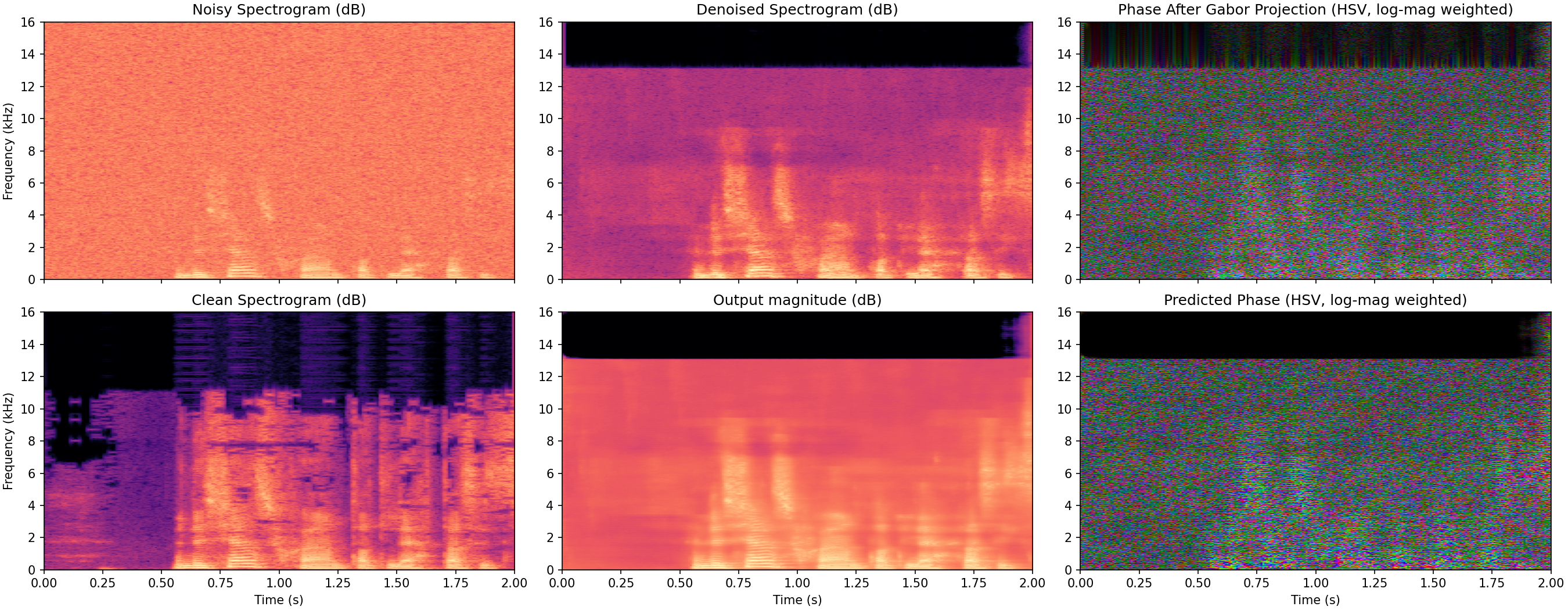
This output is arguable weaker than the two methods discussed above. Not optimizing end to end with the spectrogram $L^1$ loss certainly hurts us with this method which is a consequence of our two stage approach. A phase integrator could be made differentially to improve on this. However the big upside of the entire phase gradient approach is the ability to act in the "correct" space for audio where there are less limitations to how good the implementation can become.
Conclusions
We have looked at three increasingly complex and phase-dependent methods of reducing noise in audio using a U-Net acting on STFT-based input. Treating phase is a nontrivial but very important issue in this setting. It is a general fact of life that more intricate models are harder to train but can also perform better when done so properly. In our examples, it is not clear that, e.g., the phase gradient method performed better. Those are the types of results being shown in the papers on these methods. The goal here has instead been to show the reader some of the underlying principles at play and how they can be attacked. The implementation for all the models and plots in this post can be found on GitHub.