Notions of time-aware signal distance functions - optimal spectrogram transport
By Simon Halvdansson | Aug. 2025
Determining if two vectors are near each other is generally a straightforward problem - Euclidean distance or cosine similarity are standard solutions. In this post, we are interested in the special case where the vector indices indicate time, i.e., vectors which represent time series data or signals. There are specialized metrics available for this class of vectors but as we will see their preference for translations over modulations poses an issue for signals which exhibit some form of time-frequency structure or time-varying oscillations such as those related to audio, radar, EEG, seismic activity or vibrations.
We will make the case that an appropriate solution is optimal transport distance between spectrograms through examples where other methods fail.
Figure: Euclidean $\ell^2$, dynamic time warping and optimal spectrogram distances for a family of sinusoids of increasing frequency.
We will go over the problems with naive Euclidean $\ell^2$ distance, the standard solution which is called dynamic time warping (DTW), why it does not work when frequency changes are involved, and one way to solve it using the tools from optimal transport applied to spectrograms.
Why look at distances between signals?
The standard motivation for looking at distances between signals is to perform some sort of clustering/classification/anomaly detection task. We could get around the need for a distance function by first applying some form of encoding and computing a standard distance in a latent space. In a machine learning setting, this latent representation would be the output of some neural network like in wav2vec.
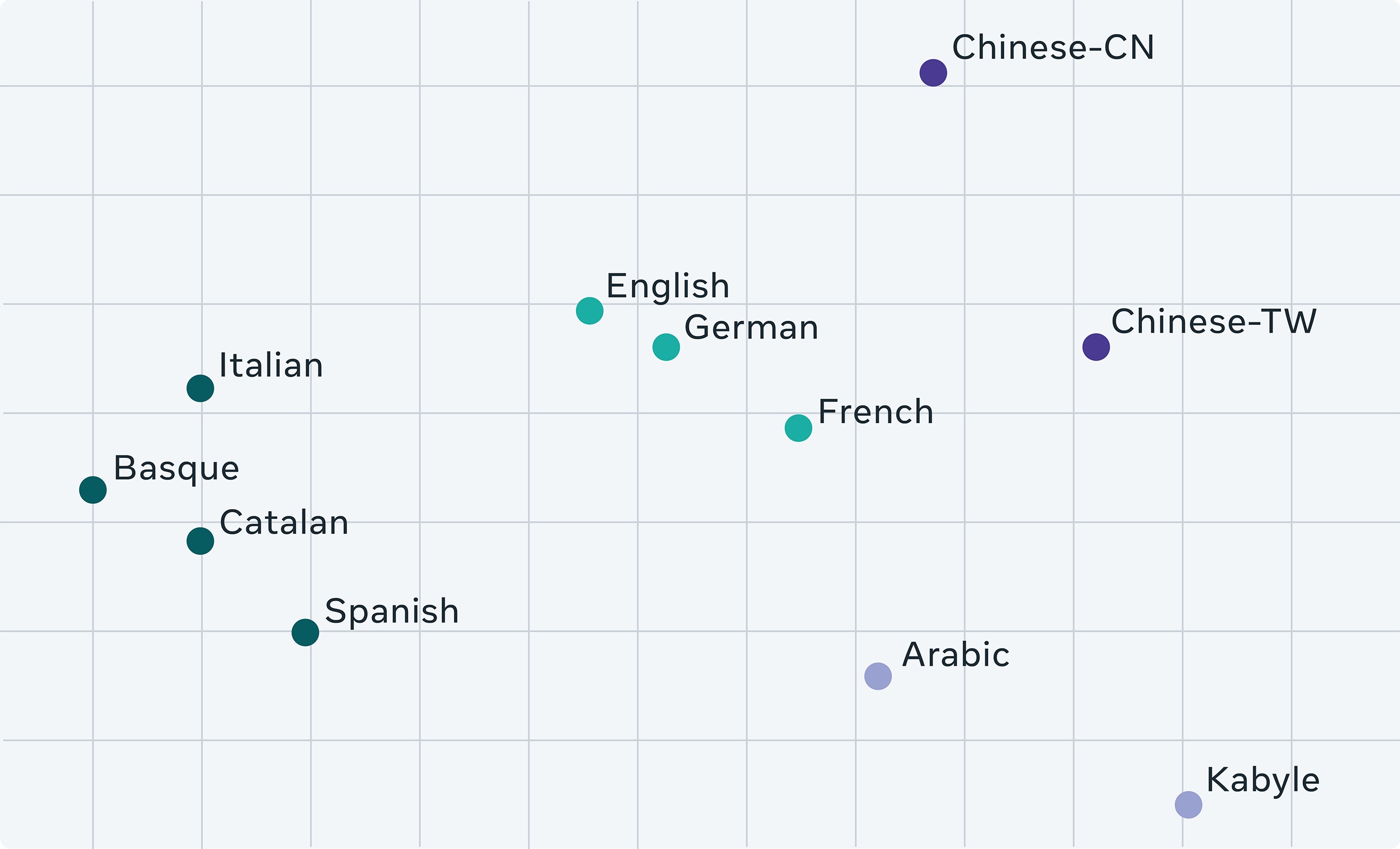
Figure: 2D PCA wav2vec 2.0 embeddings for speech audio from different languages, from the wav2vec 2.0 blog post.
There are obvious interpretability benefits to a distance function which works directly on the signal - it should be considerably more explainable than a neural encoding. A distance function which makes sense for the domain of the data also ideally should improve the inductive bias of the model and help reduce complexity of a neural network working on it.
The problem with Euclidean distance
From a time-frequency perspective there are two insurmountable problems with looking at Euclidean distance between signals (one in time, one in frequency), both best explained by examples. Consider first the case of two signals, each with a well localized peak at slightly different locations. A (low-dimensional) one would be $x_1 = (0,0,0,1,0)$ and $x_2 = (0,0,1,0,0)$. Clearly the Euclidean distance between these two vectors is $2$ but they are considerably closer than $(1,0,0,0,0)$ and $(0,0,0,0,1)$ as any sane person should conclude. Note that this is not necessarily the case if the indices do not have some temporal meaning.
The other problem with Euclidean distance is a direct corollary of Parseval's identity and boils down to pure tone sinusoids being orthogonal. This means that a 101 Hz pure tone and a 200 Hz pure tone both have the same distance to a 100 Hz pure tone. Mathematically,
$\big\langle \sin(n\,\cdot), \sin(m\,\cdot)\big\rangle = \begin{cases} 1\qquad m=n,\\ 0 \qquad m \neq n \end{cases}$
for integers $m, n$. This is what is illustrated in the figure at the start of the post.
Dynamic time warping (DTW)
Romain Tavenard wrote an excellent overview of DTW which I will refer to for details. On a high level, the dynamic time warping distance between two signals $x_1$ and $x_2$ is realized by minimizing the Euclidean distance between $x_1$ and $x_2$ over all non-decreasing index permutations. The figure below illustrates the concept nicely.
Figure: The DTW distance between two signals illustrated by the permutation map.
This is the "standard" smart solution but as we will see in the examples below, rearranging the indices does not allow us to align signals with close frequencies.
Optimal transport
For optimal transport, sometimes called the earth mover's distance or Wasserstein distance, the underlying idea is to consider how much work it is to go from one distribution to another, both of the same mass. In the simplest case where the two distributions are point masses, this required work is equal to the distance between the two points. For more complex densities $\mu, \nu : X \to \mathbb{R}$, a transport plan $\pi : X \times X \to \mathbb{R}$ tells us how much mass to move for each pair of points. In order to preserve mass, this means that for any point $y$, the mass of $\nu$ at $y$, $\nu(y)$, must match the mass which is moved from all of $X$ to $y$, i.e., $$\nu(y) = \int_X \pi(x,y)\,dx.$$ Moreover, the mass which leaves a point $x$ is precisely $\mu(x)$, i.e., $$ \mu(x) = \int_X \pi(x,y)\,dy. $$ There can be many such transport plans but the optimal transport distance is the minimal cost $\int_{X \times Y} |x-y| \pi(x,y)\,dx\,dy$ over all possible transport plans. The concept is most easily demonstrated by an animation like in the following figure.
Figure: Continuous morphing along straight lines for an optimal transport plan between two distributions. Dottiness is a consequence of numerical inexactness.
There are extensions where we can punish distance nonlinearly or differently depending on the axis but for the purpose of this post we can think of it as the sum of all the distances moved multiplied by the mass moved at each point.
Optimal spectrogram transport
The spectrogram of a signal is a 2-dimensional representation, meaning a function $\mathbb{R} \times \mathbb{R} \to \mathbb{R}$, where the axes represent time and frequency. It should be thought of as a series of spectra (absolute value of Fourier transform) for small time snippets of the full signal, ordered in increasing time along the $x$-axis. In the following figure, we show an example of a spectrogram of a signal which changes its frequency contents over time to illustrate the concept.
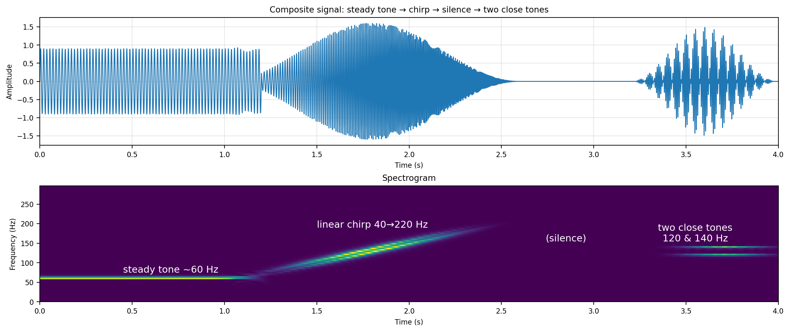
Figure: Signal and associated spectrogram for a signal which goes from steady tone to chirp to silence to two close tones.
Now the idea behind optimal spectrogram transport is that the optimal transport distance between spectrograms should capture most of what we intuitively think of as distance between signals of this kind. Below we have chosen a slightly modified version of the above signal (different steady tone, reversed chirp, two tones moved and modulated) and illustrate the optimal transport interpolation between them.
Figure: Optimal transport morphing between spectrograms of two similar signals with slightly different characteristics.
This is how we define optimal spectrogram transport distance. Note that there exists fast algorithms and libraries for computing optimal transport with GPU acceleration but even on a CPU this computation is feasible in a real-time setting.
Examples
For all our examples, we will consider families of functions indexed by some continuous variable which intuitively should result in a continuously increasing distance. The first such example is for a modulated Gaussian, $f(x) = \sin(x) e^{-x^2}$, which we dilate using a dilation parameter $a$. A nice distance function should then satisfy $$ d(f_{a_1}, f_{a_2}) \propto |a_1 - a_2| $$ where we mean proportionality in a loose sense. In the figure below, we have signals and spectrograms for three such dilations and the continuous functions $d(f_a, f_1)$.
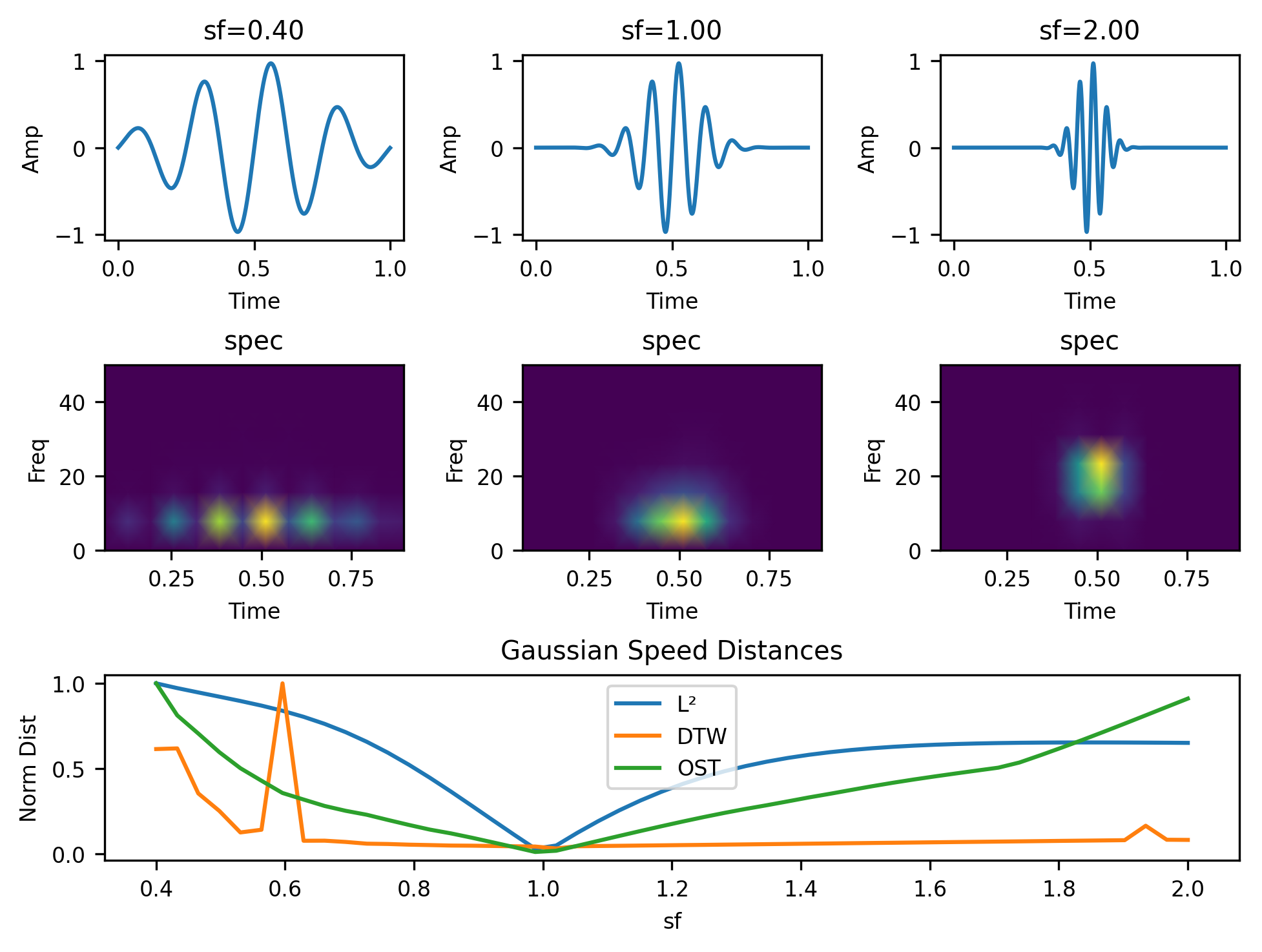
Figure: Euclidean $\ell^2$, dynamic time warping and optimal spectrogram distances for a family of modulated Gaussians with varying dilations.
In this case, Euclidean distance works okay for small dilations but plateaus for larger ones, while dynamic time warping is mostly flat. Meanwhile optimal spectrogram transport distance behaves like we want it to and continues increasing as the dilation parameter moves away from $1$.
The GIF in the beginning of the post covered how the metric is continuous with respect to modulations. We compare continuity with respect to translations in the following example.
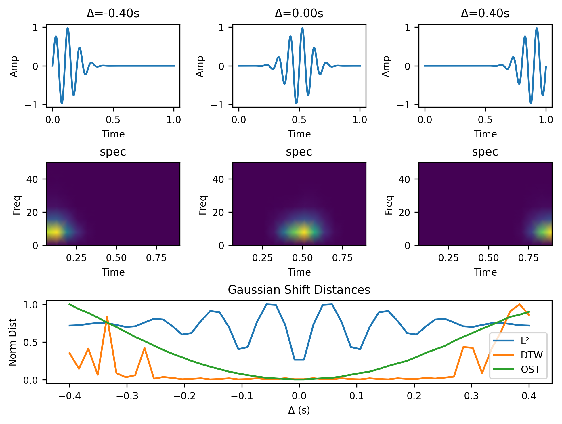
Figure: Euclidean $\ell^2$, dynamic time warping and optimal spectrogram distances for a family of modulated Gaussians with varying translation.
Again, the behavior of optimal spectrogram transport is preferable to that of both Euclidean and dynamic time warping distance.
Lastly we consider the case of continuity with respect to noise level which all the different metrics handle well.
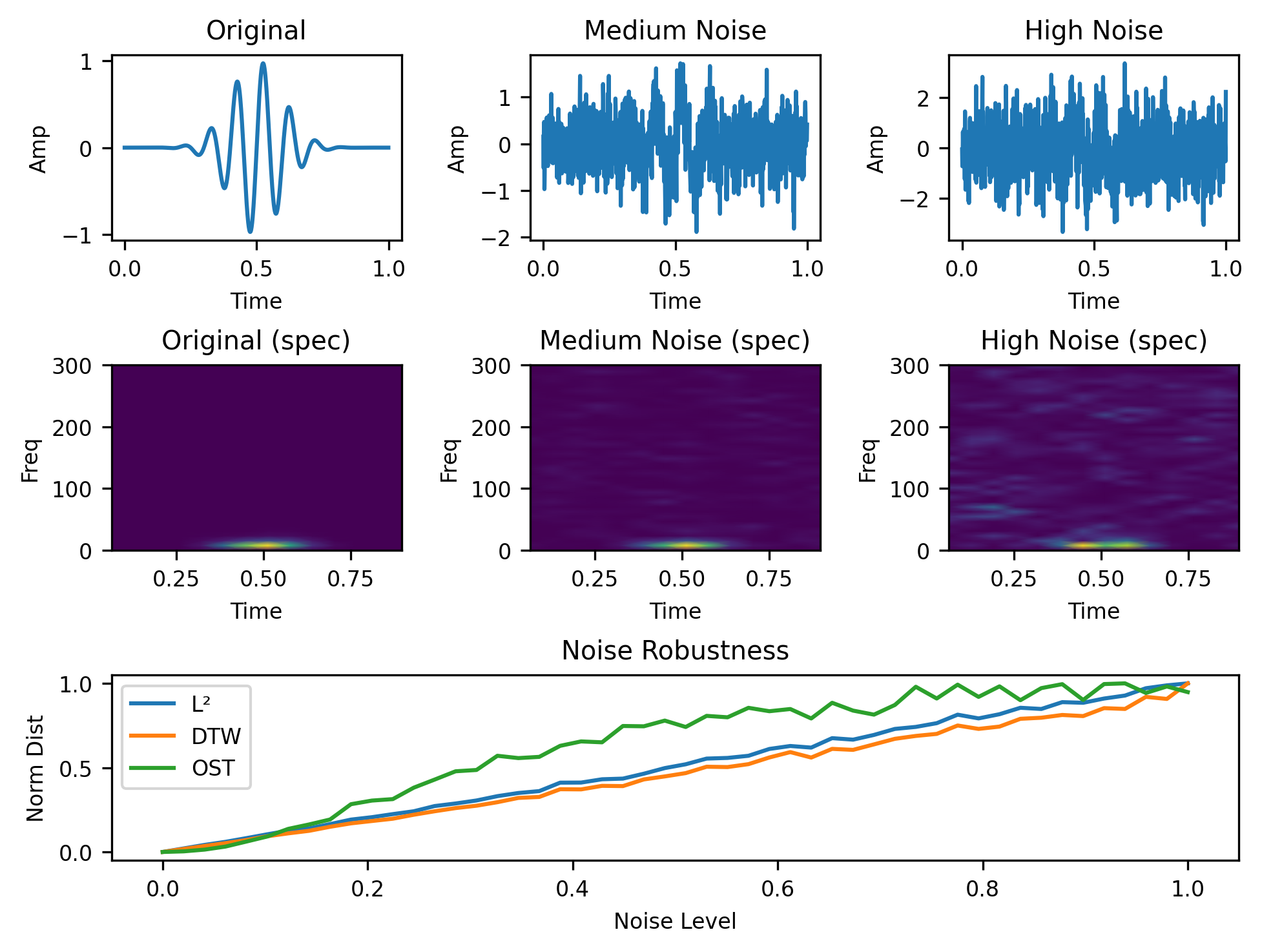
Figure: Euclidean $\ell^2$, dynamic time warping and optimal spectrogram distances for a family of modulated Gaussians with varying noise levels.
Closing remarks
Optimal spectrogram transport is an idea which I've had in my head for many years and hopefully this post has convinced you that it's an obvious next step once you've learned about spectrograms, optimal transport and the issues of other metrics. In the process of preparing this post I found some other recent work in this direction and hope that this is an idea which continues to be explored.