Vibe-GPU-accelerating a 2D particle simulator from mathematical physics

In 2019, as part of my Bachelor's thesis, I wrote a simple 2D particle simulator for a certain system in mathematical physics called the 2D Coulomb gas with a remarkable amount of theory behind it. I've always wanted to add GPU acceleration to this simulation but prospects were even worse back then with WebGL / WebGL 2.0 being the standard solutions for utilizing the GPU on the web. Recently, after trying for several years, I was able to get an LLM to do this conversion and an updated version of the simulator is now live. In this post, I'll discuss the simulator and the problem in limited detail.

I encourage you to try the simulators out briefly before continuing on. Either way, the problem we are interested in shows up in several different contexts but they one I find easiest to follow is the physical one with charged particles. Consider a collection of $n$ electrons in the 2D plane, all experiencing pariwise Coulomb repulsion. Such a system has a fairly predictable behavior of spreading out across the plane as time progresses. To make this system a bit more interesting, we can add a electrical potential which goes to infinity far out on the plane. With these counteracting forces, we stand a chance of obtaining a stable system, provided the potential is chosen appropriately.

It can be worked out that in 2D, Coulomb repulsion between charged particles is proportional to the logarithm of the distance between the particles. With this, we can write the Hamiltonian (total energy) of the system with appropriately chosen constants as $$ H_n(z_1, \dots, z_n) = \sum_{i \neq j} \log \frac{1}{|z_i - z_j|} + n\sum_{j=1}^n Q(z_j) $$ where $z_1, \dots, z_n \in \mathbb{R}^2$ are the locations of the particles. Note that the number of terms in the first sum is proportional to $n^2$ which is why we have added the factor $n$ to the second sum.

In studying the Coulomb gas, we are generally interested in random realizations of this system in the sense of statistical mechanics, meaning that the probability of observing a single configuration $(z_1, \dots, z_n)$ is proportional to $\exp(-\beta H_n(z_1, \dots, z_n))$ where $\beta = 1/T$ is the inverse temperature of our system. Generally, we fix $\beta = 1$ for simplicity.

Ginibre ensemble

As a quick aside, we will discuss the prototypical example of interaction between the 2D Coulomb gas and another field, namely random matrix theory, in the form of the Ginibre ensemble. This is the case of $Q(z) = |z|^2$ which turns out to precisely correspond to the eigenvalues of a random matrix with complex $\mathcal{N}(0,1/\sqrt{n})$ entries. Here we need to identify points of $\mathbb{R}^2$ with points of $\mathbb{C}$ in the classical way $(x, y) \sim x+iy$. If we then run

import numpy as np

n = 100
A = (np.random.randn(n, n) + 1j*np.random.randn(n, n))/np.sqrt(2*n)

eigvals = np.linalg.eigvals(A)

and plot the results, we get the following type of plots:

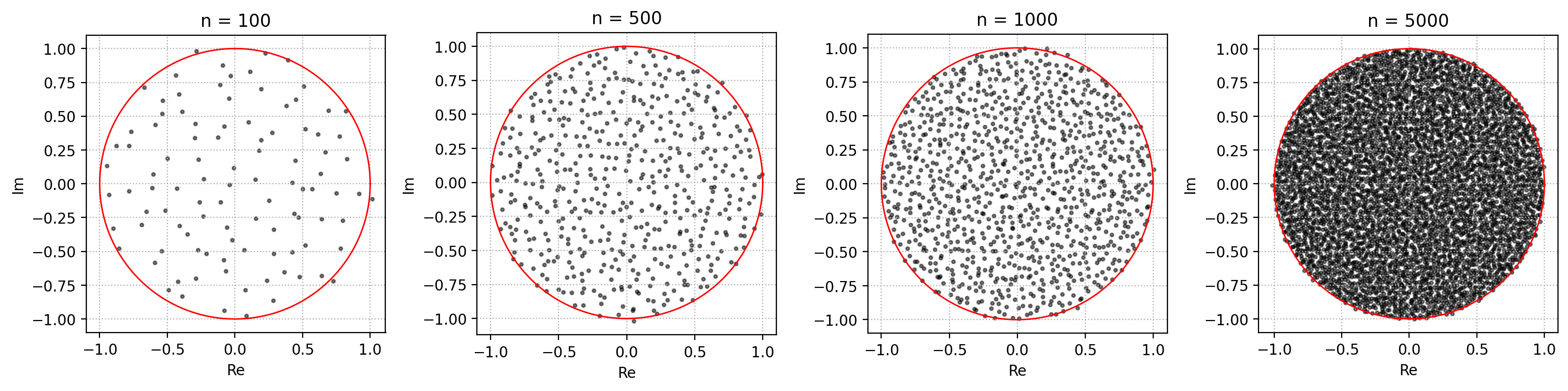
Note that the eigenvalues generally tend to fall in the unit disk, boundary indicated in red in the figure. This is a special case of the universal behavior that eigenvalues tend to occupy a certain compact subset of the plane called the droplet $S$ with density proportional to $\Delta S$. In the case of the Ginibre ensemble, $\Delta Q \equiv 1$ which explains the even spread of the points within the unit disk. We won't say more about the underlying theory but remark that we truly have just scratched the surface and the thesis has a longer introduction.

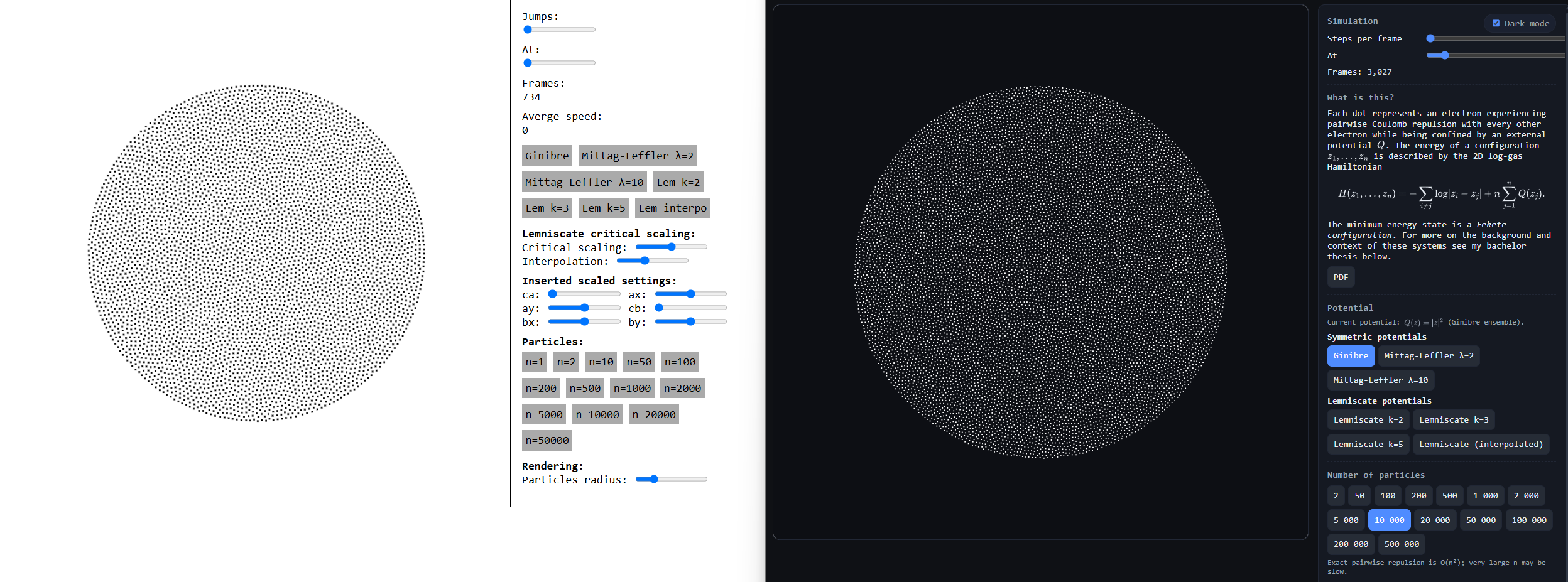
Simulator

Actually sampling the joint probabilities induced by the $\exp(-\beta H_n)$ law is extremely expensive so if you want to get a feel for the behavior of the points without breaking the bank, treating the points as actual charged particle subject to the forces induced by our Hamiltonian is a great solution. As you might have guessed, this is equivalent to minimizing $H_n$ using gradient descent. Note that $\beta \to \infty$ corresponds to the minimum energy configuration and $\beta \to 0$ corresponds to an increasingly random configuration with variance going to $\infty$.

On a related note, simulating the 2D Coulomb gas is similar to the Thomson problem in which there is no external potential but the particles are instead restricted to the unit sphere and the goal is to find the minimum energy configuration. I was interested in this problem long before learning of statistical mechanics and the 2D Coulomb gas and had already written a super simple simulator for it which inspired the simulator for the 2D Coulomb gas.

Either way, this first simulator worked fine and I used it to generate some visualizations for the thesis by leaving the computer running overnight. The speed certainly leaves something to desire but it's fast enough that you can (mostly) run it with 50,000 particles without the Chrome tab crashing. The pairwise repulsion leads to a $O(N^2)$ runtime and the need for precision to conform to the theory means that we cannot make do with approximations.

WebGPU conversion

After the thesis, I tried my hand at converting to code to run using first WebGL and later WebGPU but without sufficient motivation, this proved difficult. Still, this seemed like just the type of tedious work which LLMs should be able to complete. With new model releases, I tried my hand at this and at one point Claude Sonnet had an almost working version but it wasn't until GPT-5 that this could be solved in a sufficiently nice way. The result turned out really nice and I ended up making some quality of life improvements as well.

I might build something extra onto the simulator in the future but until then I'm really happy with how the project turned out. With modern LLMs it is so much easier to make programs to verify or visualize research and I hope this practice is much more common in the future.