Implicit neural representations of images are quick learners
Implicit neural representations (INRs) aim to encode functions between low dimensional spaces such as audio signals, images, 3D models or videos by means of a neural network. The field is evolving rapidly but is still relatively nascent with some variability in the architectures used. While there has been some survey work which is good for an overview, in this post we provide a deeper investigation about how to set up the MLPs and talk about possible improvements (mixture-of-experts, LayerNorm and skip connections). We find that with some good choices it is possible to learn an image with an INR in mere seconds with excellent performance and talk about some of the implications of this.
Our findings may be summarized as follows:
- With enough parameters, an INR can learn an image with negligibly small error in seconds.
- The standard ReLU activation function appears to be optimal when using feature mappings.
- Hyperparameters like learning rate and optimizer can have very different behavior for different images.
- MoE, while expensive parameter-wise, can indeed improve performance both at fixed compute budgets and for longer training
- LayerNorm is very strong for improving convergence speed and training stability when used with a standard MLP
- Skip connections do not seem to help either convergence
The benchmark problem
We choose to focus fully on INRs of images to reduce the amount of work, meaning that we learn functions $I : [0,1]^2 \to [0,1]^3$ where $(x,y) \mapsto (r,g,b)$. Specifically, let $\mathcal{N}$ be a neural network. We then choose something like mean squared error as our loss function meaning that we minimize
To get a comparison which has hopes of generalizing, we choose a collection of 5 images, each of resolution 768×768 pixels. Our error metric will be the standard peak signal-to-noise ratio (PSNR) since this is often used in papers when comparing models. To keep the comparison fair, we train the models for 3 minutes per image. This seems to be in line with or less than the typical training time used in papers.


This is the problem we will hill climb, and we leave questions about its suitability and the implications to the end. Before going into the results, we briefly go over what our models look like.
INR models
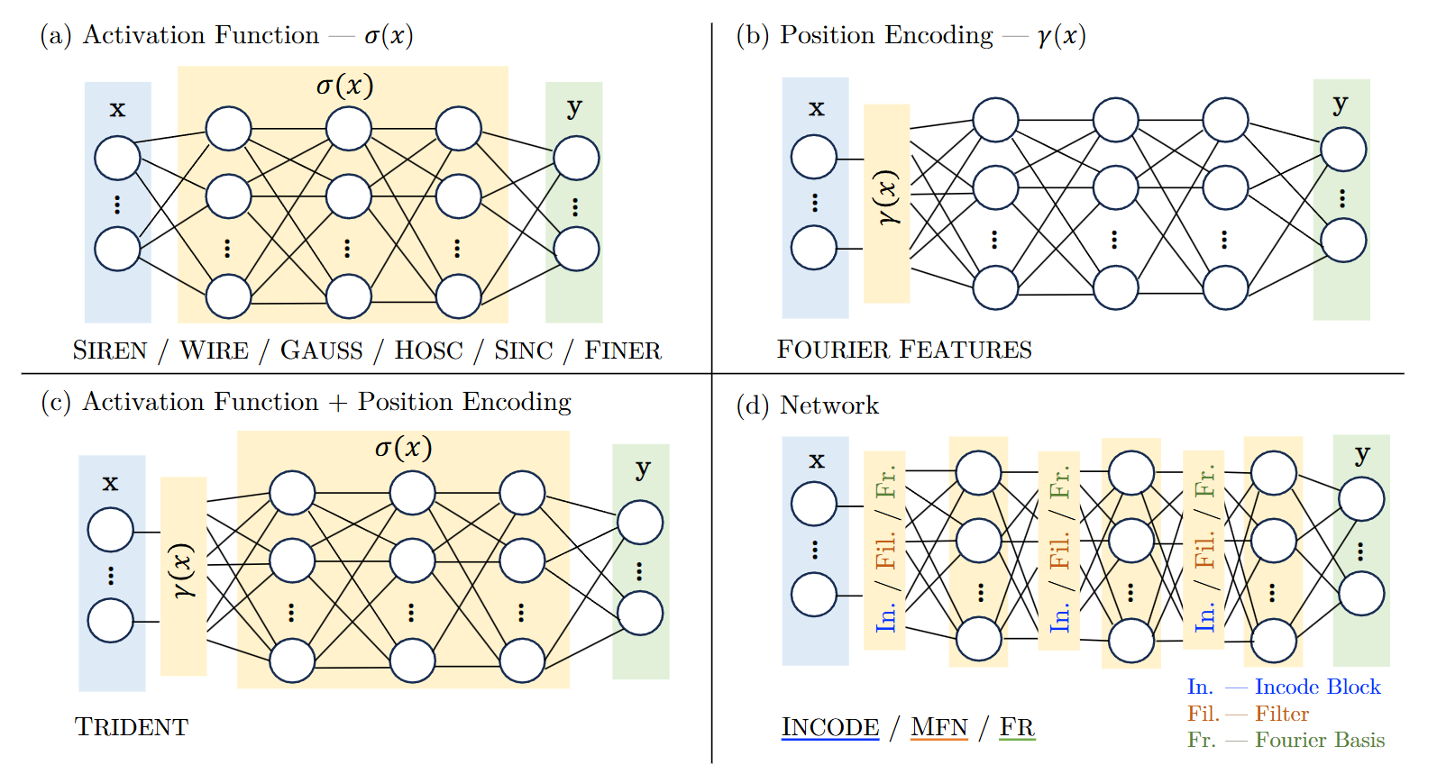
We will limit ourselves to a more classical set of architectures for our INRs. Specifically, we will only deal with a position encoding step followed by an MLP which we allow for some freedom over. In the language of the INR survey mentioned earlier, this means that we modify the yellow parts of (c) in the figure below.
Position encoding
Formally, our neural network then has the form $\mathcal{N}(x) = \operatorname{MLP}(\gamma(x))$. For the feature encoding $\gamma$ we will consider Fourier features and Gabor features, discussed in an earlier post. In PyTorch we write these as follows:
class FourierFeatures(nn.Module):
    def __init__(self, input_dim, dim_per_input=20, freq_scale=None, trainable=False):
        super().__init__()

        if freq_scale is None:
            freq_scale = 0.5*dim_per_input/torch.sqrt(torch.tensor(2 * torch.pi))

        freqs = torch.randn(input_dim, dim_per_input) * freq_scale

        if trainable:
            self.freqs = nn.Parameter(freqs)
        else:
            self.register_buffer('freqs', freqs)

    def forward(self, x):
        phase = 2 * torch.pi * (x @ self.freqs)
        return torch.cat([torch.cos(phase), torch.sin(phase)], dim=-1)

class GaborFeatures(nn.Module):
    def __init__(self, input_dim, dim_per_input=20, freq_scale=None, trainable=False):
        super().__init__()

        if freq_scale is None:
            freq_scale = 0.5*dim_per_input/torch.sqrt(torch.tensor(2 * torch.pi))

        centers = torch.rand(dim_per_input, input_dim)
        freqs = torch.randn(dim_per_input, input_dim) * freq_scale
        sigmas = torch.full((dim_per_input, input_dim), 0.1*torch.sqrt(torch.tensor(256/input_dim)))

        if trainable:
            self.centers = nn.Parameter(centers)
            self.freqs = nn.Parameter(freqs)
            self.sigma = nn.Parameter(sigmas)
        else:
            self.register_buffer('centers', centers)
            self.register_buffer('freqs', freqs)
            self.register_buffer('sigma', sigmas)

    def forward(self, x):
        diff = x.unsqueeze(1) - self.centers.unsqueeze(0)
        envelope = torch.exp(- (diff ** 2 / (self.sigma.unsqueeze(0) ** 2)).sum(dim=2) / 2)
        phase = 2 * torch.pi * (diff * self.freqs.unsqueeze(0)).sum(dim=2)

        return torch.cat([envelope * torch.cos(phase), envelope * torch.sin(phase)], dim=-1)
Note that when using position encodings, we have here exposed the parameter trainable for if the frequencies, centers and widths should be viewed as parameters or fixed but random parameters, freq_scale for how we sample the frequencies and dim_per_input which yields the output dimension input_dim × dim_per_input. This opens up a lot of room for optimization.
MLP
For the MLP backbone, we expose standard hyperparameters like activation function, number of layers and hidden dimension (which we take to be fixed across each layer for simplicity). However we also allow for the three less standard extensions mentioned in the introduction, namely mixture-of-experts (MoE), skip connections and LayerNorm.
For the MoE, we pass the raw coordinates through a small gating network with an output of length n_experts which is softmaxed. Then n_experts MLPs treat the positional encoding output to produce pixel values and the results are weighted by the gating outputs before being sigmoided:
def forward(self, x):
	gate_logits = self.gate(x)

	x = self.pos_enc(x)

	gate_weights = F.softmax(gate_logits, dim=-1)

	expert_outputs = []
	for expert in self.experts:
		y = expert(x)
		expert_outputs.append(y.unsqueeze(-2))

	expert_outputs = torch.cat(expert_outputs, dim=-2)

	mixed = torch.sum(
		gate_weights.unsqueeze(-1) * expert_outputs,
		dim=-2
	)

	return self.sigmoid(mixed)
Skip connections are handled inside the MLPs and only applied to the states of length hidden_dim with $\frac{1}{\sqrt{2}}$ weighing, i.e., x = (x + x_skip)/torch.sqrt(2). For LayerNorm preliminary investigations showed that post vs pre-norm (norm before or after activation function) had a minimal effect on performance and the same was true for LayerNorm versus RMSNorm so we keep it simple and only consider post-LayerNorm.
Training hyperparameters
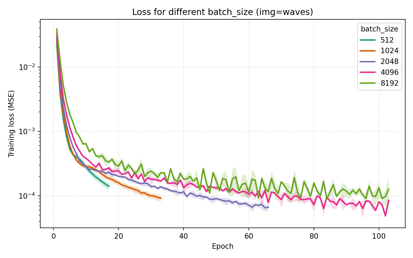
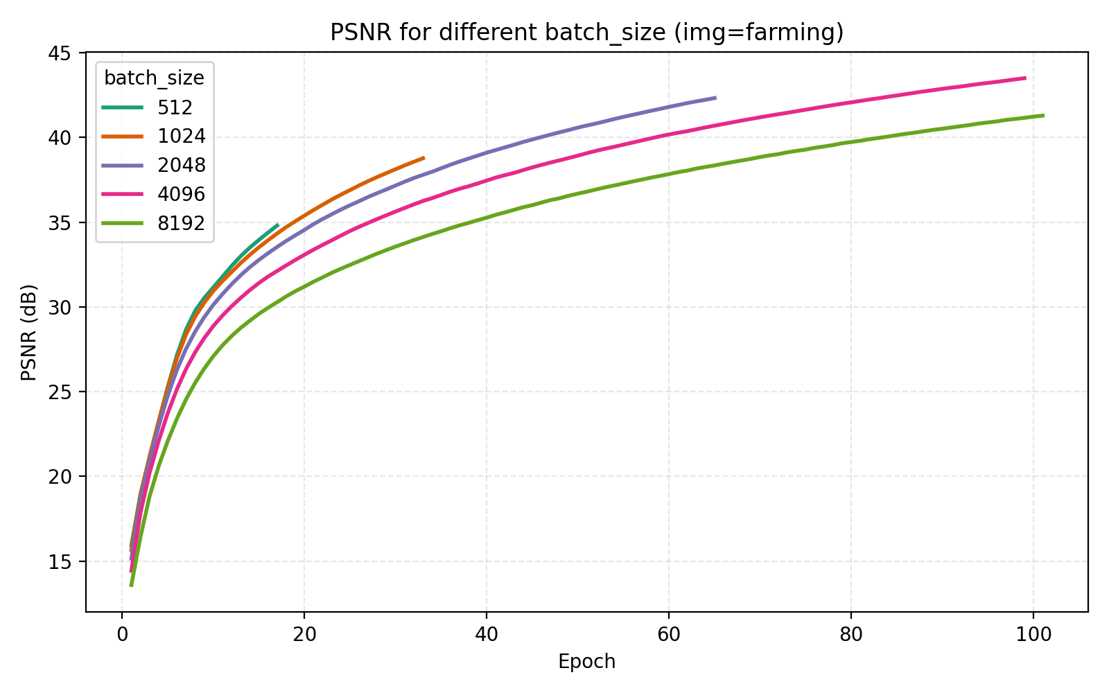
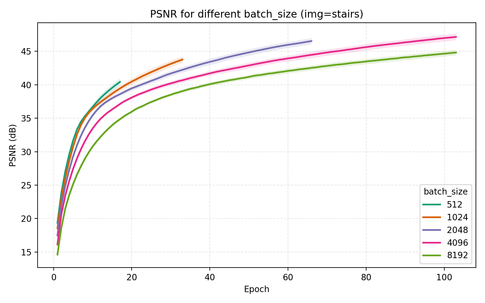
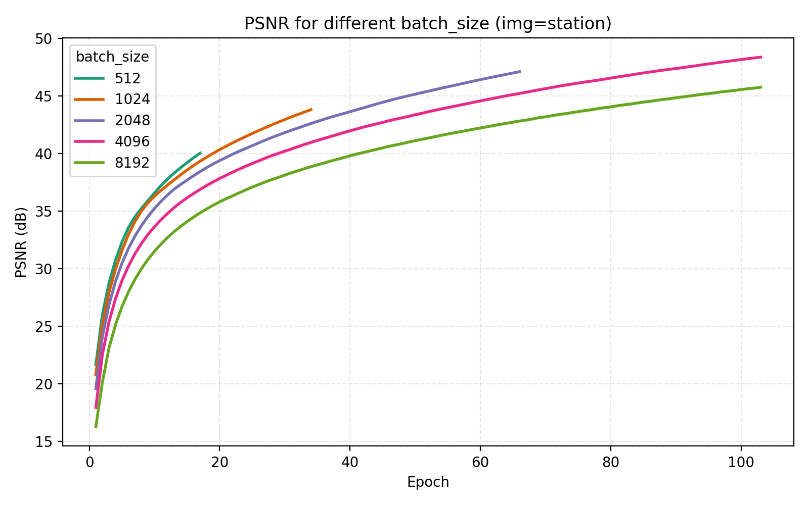
We will also look at tweaking the learning rate lr and batch size batch_size for the training.
Baseline
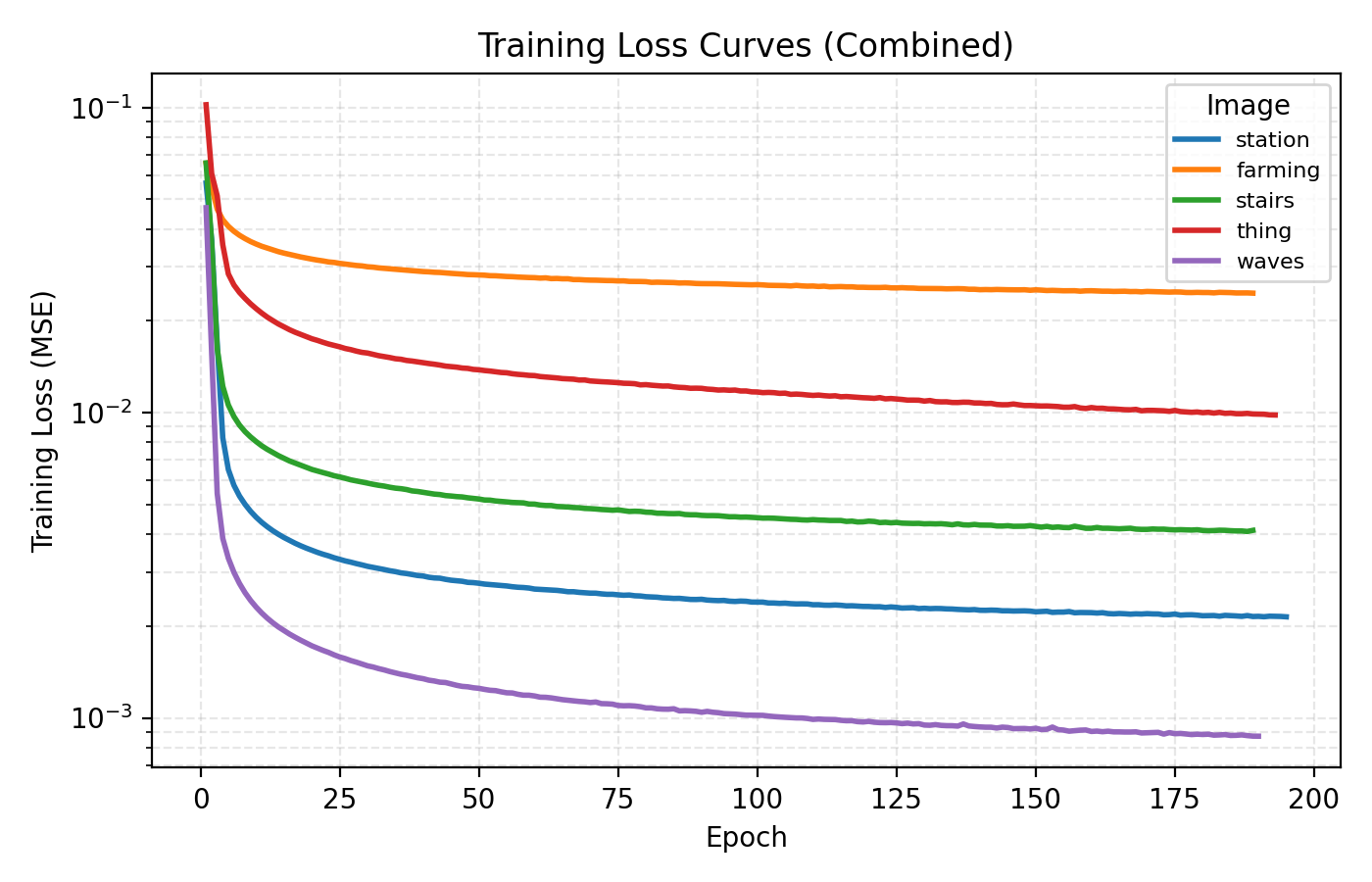
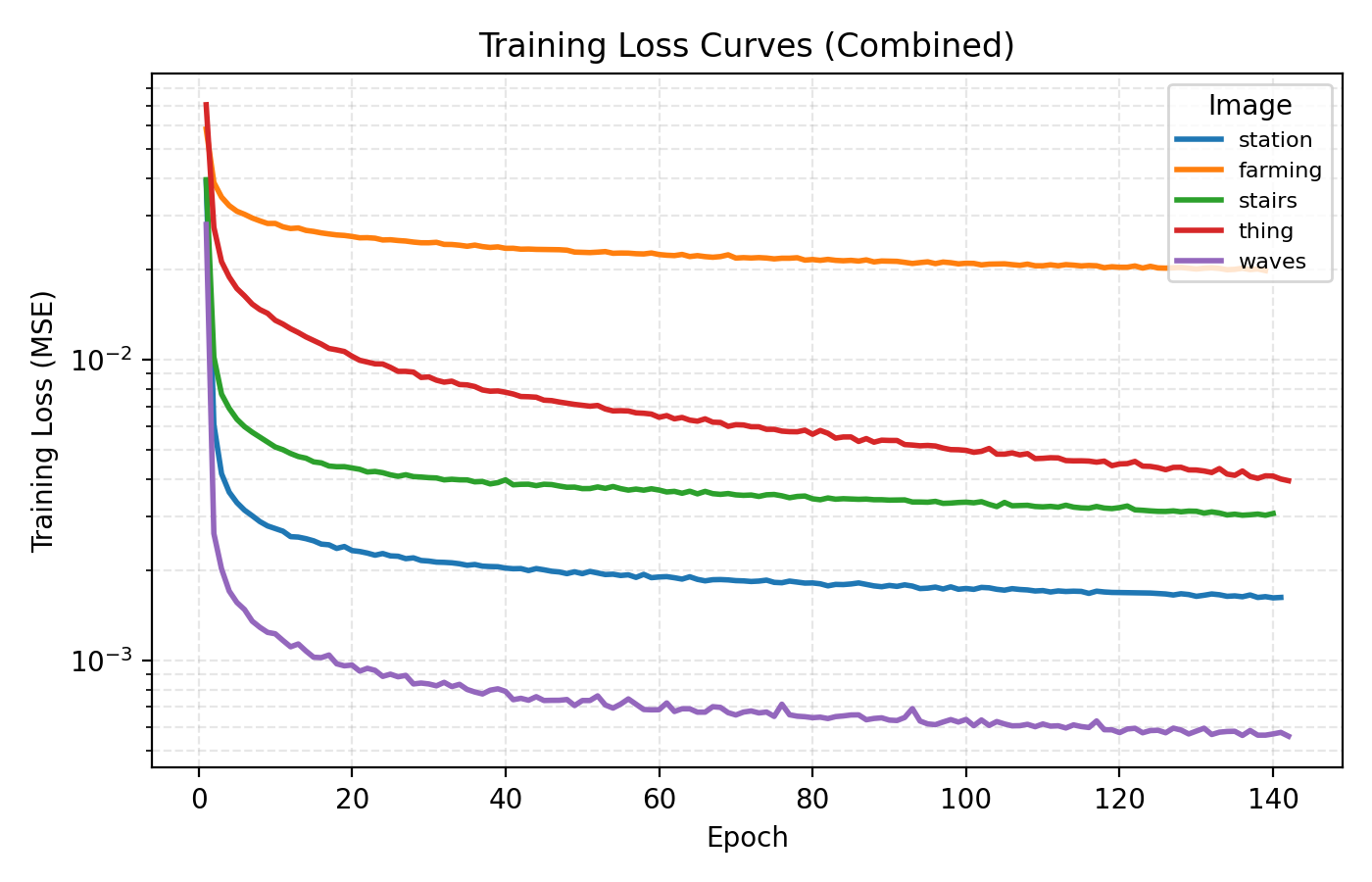
First up we train a bog standard INR with Fourier features, an embedding dimension of 64, 4 hidden layers of dimension 256 and ReLU activation for a 150k parameter model. Below are snapshots from training that network for 3 minutes per image with a learning rate of 1e-4.
In this example the loss is extremely rapidly decreasing in the start and plateaus at rather high level. However the level at which the loss curves plateau differ greatly for the different images. We see for example that the farming image is hard to learn, most likely due to its significant high frequency components.
We now move to improving this performance by using the average PSNR across these five images as our objective function.
Scaling up standard MLPs
Our first step will be to try out a larger MLP since performance seems to saturate rather quickly.
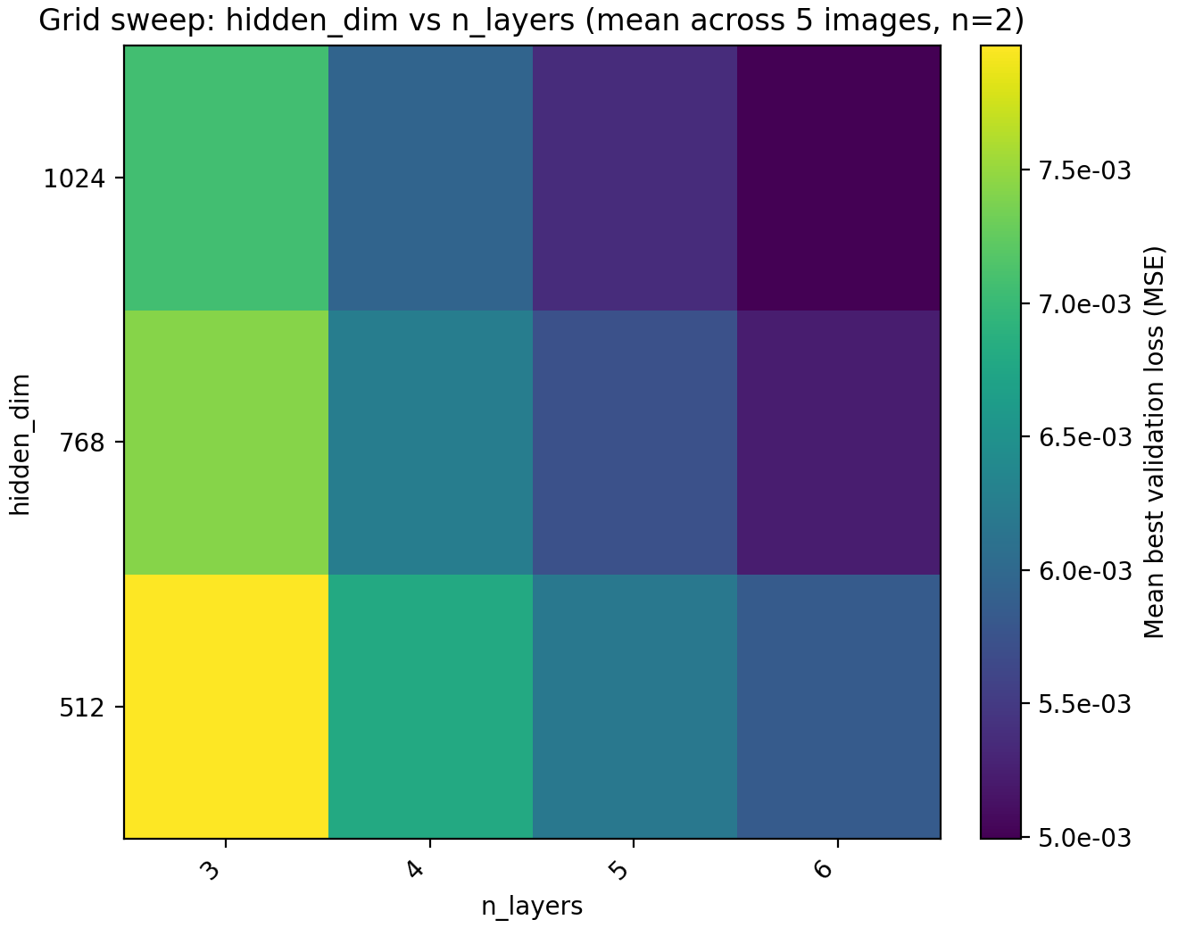
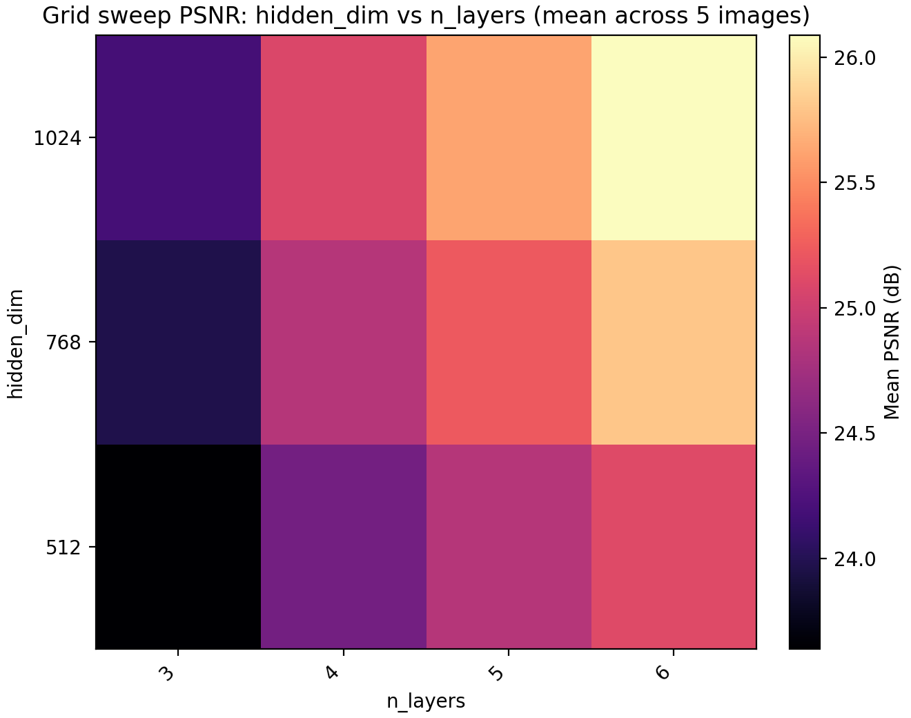
hidden_dim (x-axis) and n_layers (y-axis). The loss curves are with the optimal choice.
Based on this information we set n_layers = 6 and hidden_dim = 1024 but leave a note about trying out larger values for these later. The model now has 4.3M parameters but we remark that we have chosen to only use training time as our restriction. Obviously this is not the correct restriction if one is attempting to, e.g., compress images using an INR, in which case we would probably have a fixed parameter budget as well.
We could definitely have pushed MLP size further at this point but remark that when we have no positional encodings, we get stuck in this sort of plateau where we can get performance gains from increasing the parameter count but we are fundamentally unable to express the details of the image with it and are only digging deeper into a local minimum. For this reason we next up look at encoding dimension and frequency scale. Recall that the encoding dimension is the output dimension of $\gamma$ and the frequency scale is the standard deviation of the Gaussian which the frequencies are taken from.
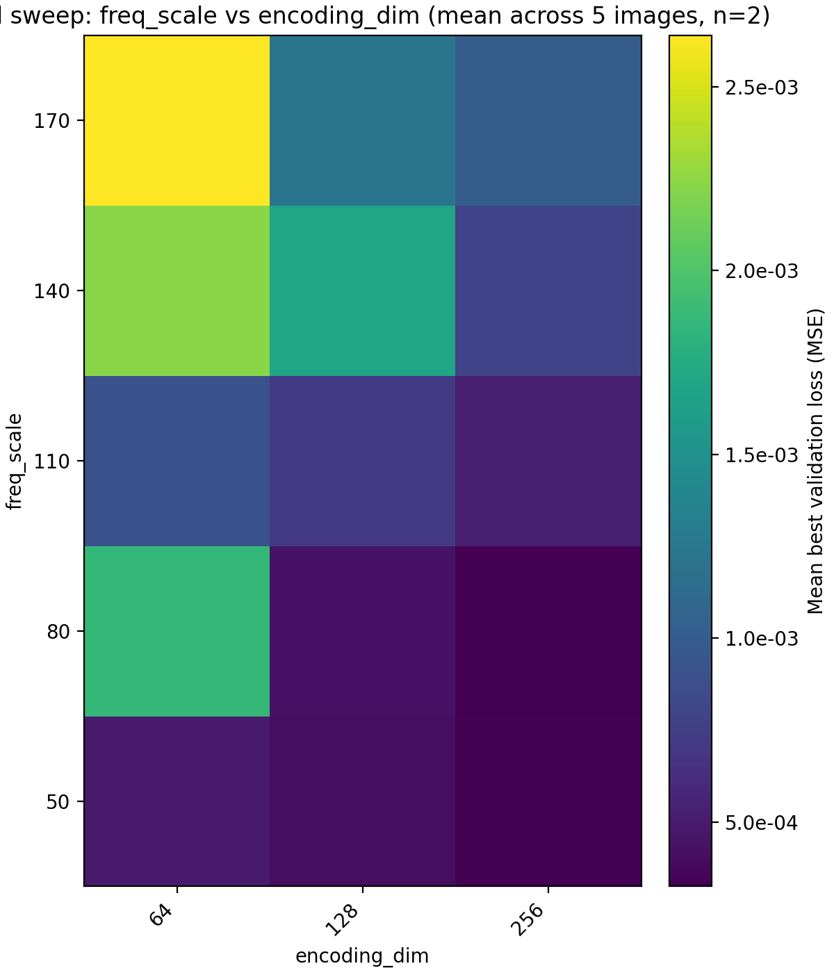
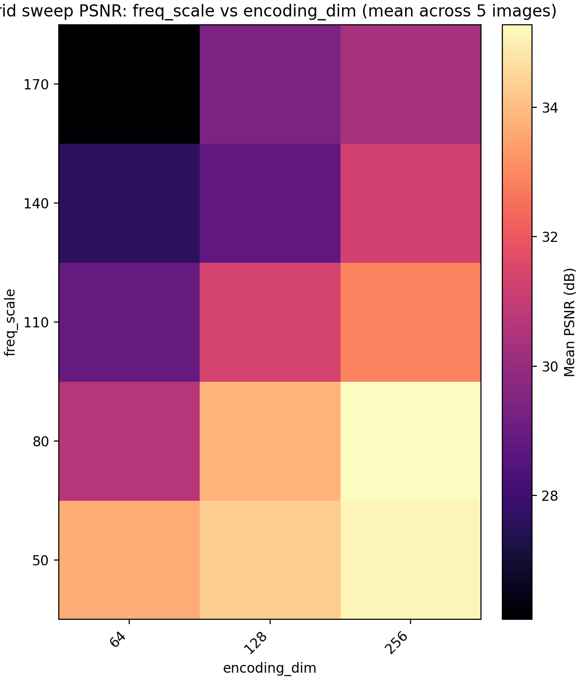
encoding_dim (x-axis) and freq_scale (y-axis).
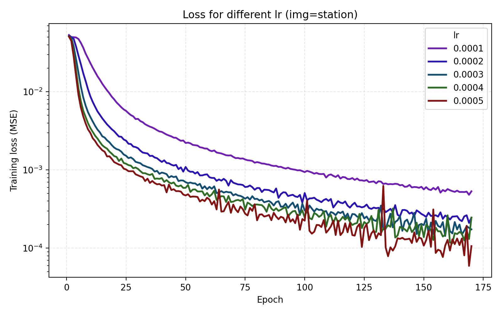
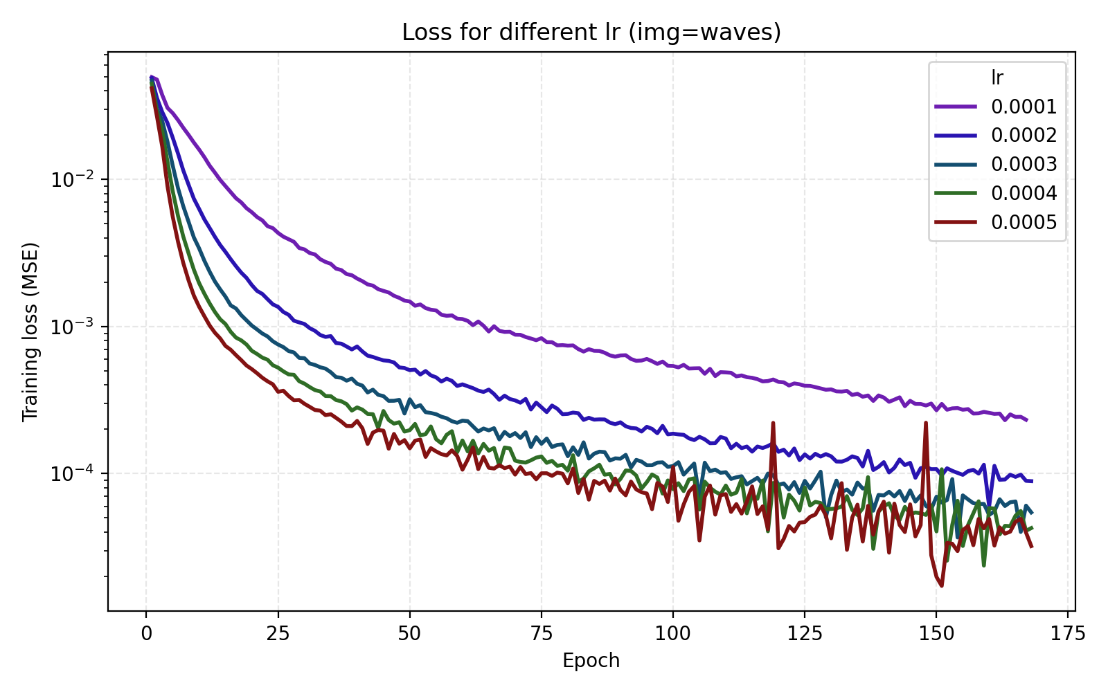
Here we get a large jump in average PSNR from 26 dB to 35 dB. Setting encoding_dim = 256 and freq_scale = 80 bumps the parameter count slightly to 4.5M. We now move to tuning the learning rate. In this case, just looking at the average MSE or PSNR does not tell the whole story since there is a large discrepancy between the images.
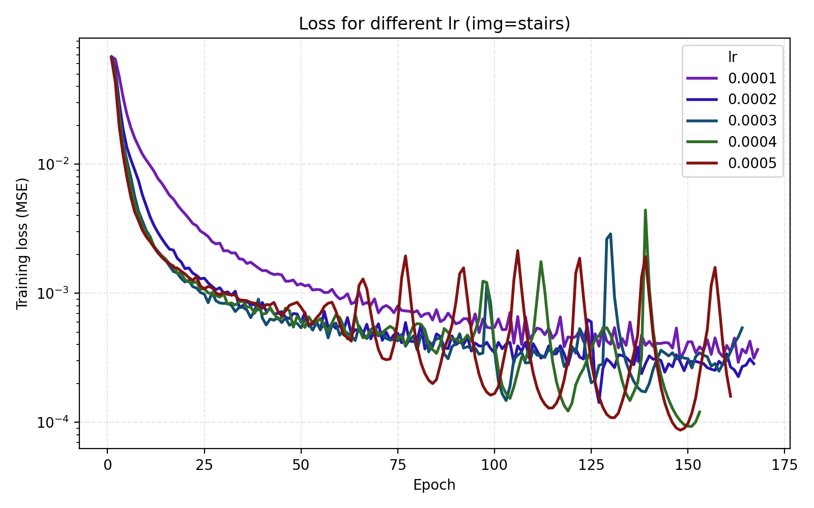
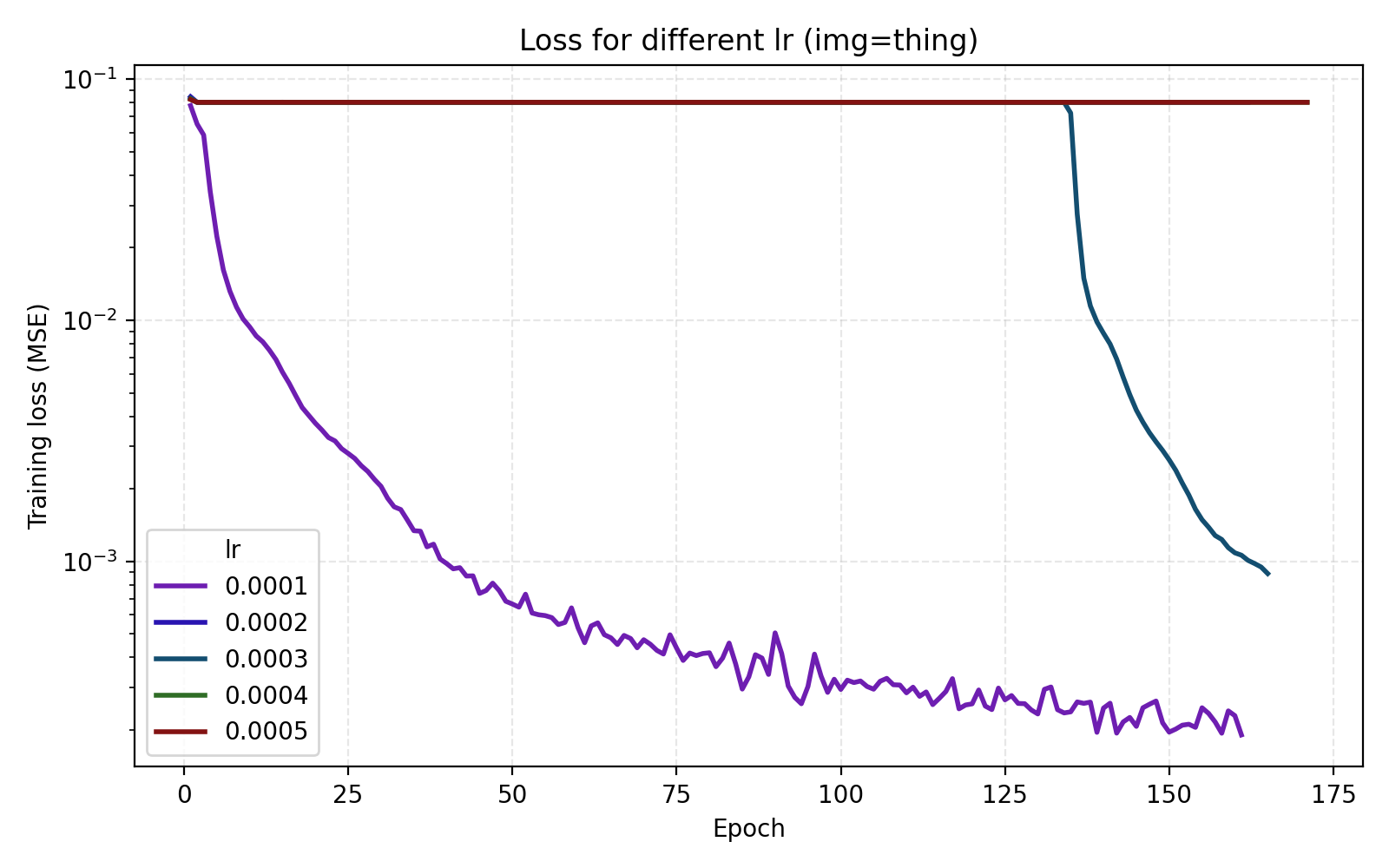
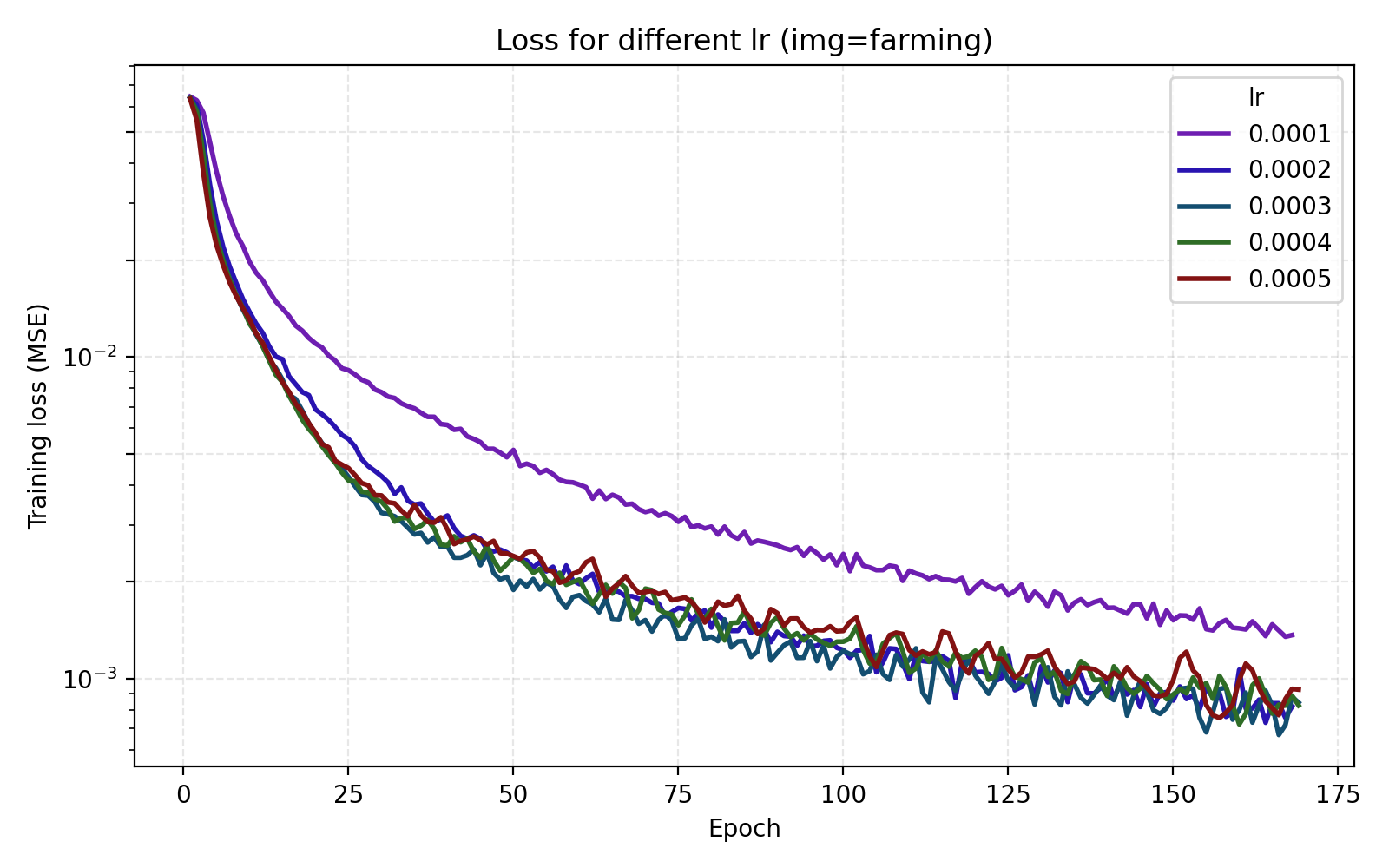
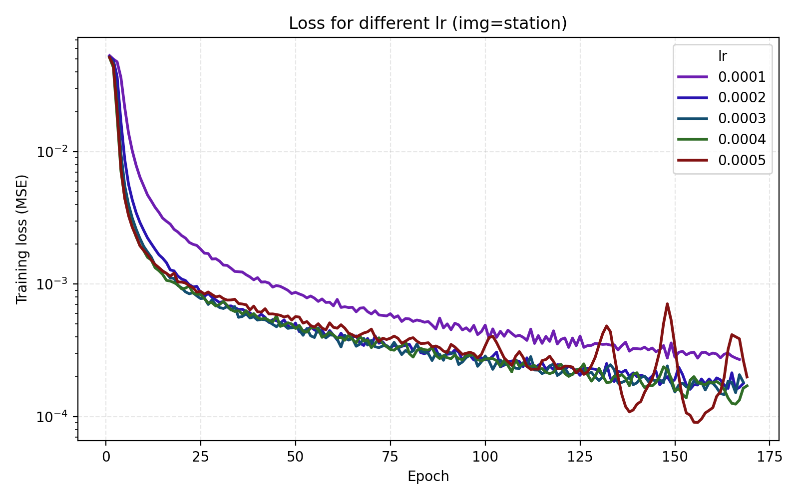
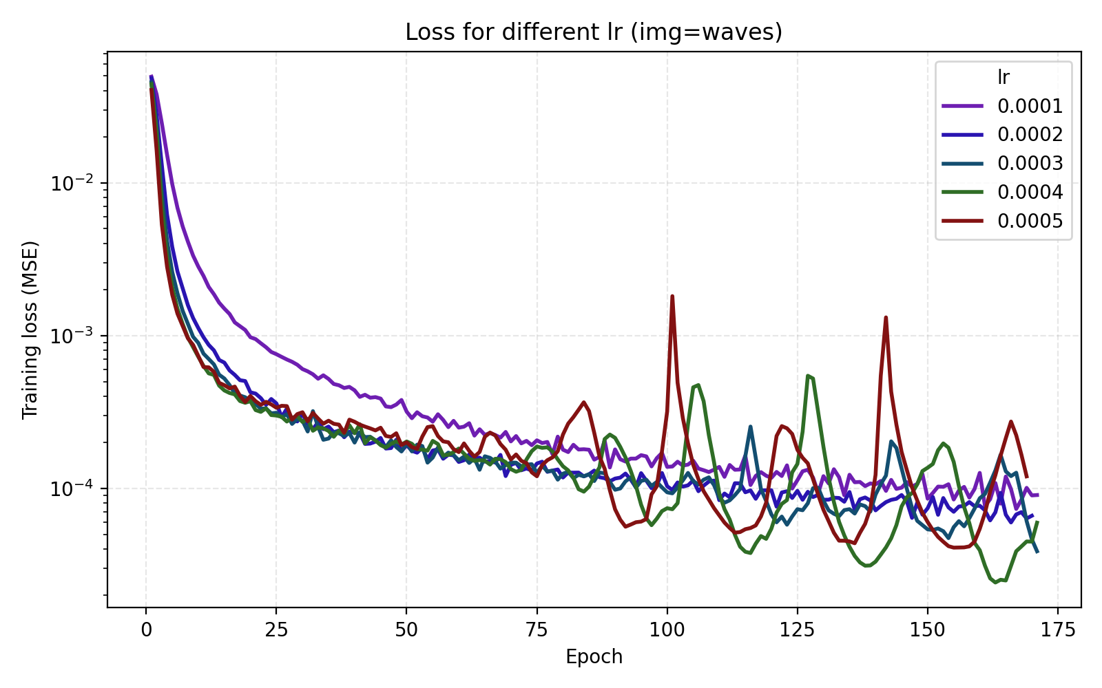
We see that stairs and thing are particularly unstable at higher learning rates. Meanwhile the arguably optimal learning rate 1e-4 for those performs poorly for the other three images. An interpretation is that learning rate can greatly benefit from being tuned for the data set (image). Since we are looking for one training recipe that is strong throughout, we instead try the ScheduleFree version of AdamW. This is an optimizer which is supposed to be more adaptive than vanilla AdamW which is what we also see in our results.
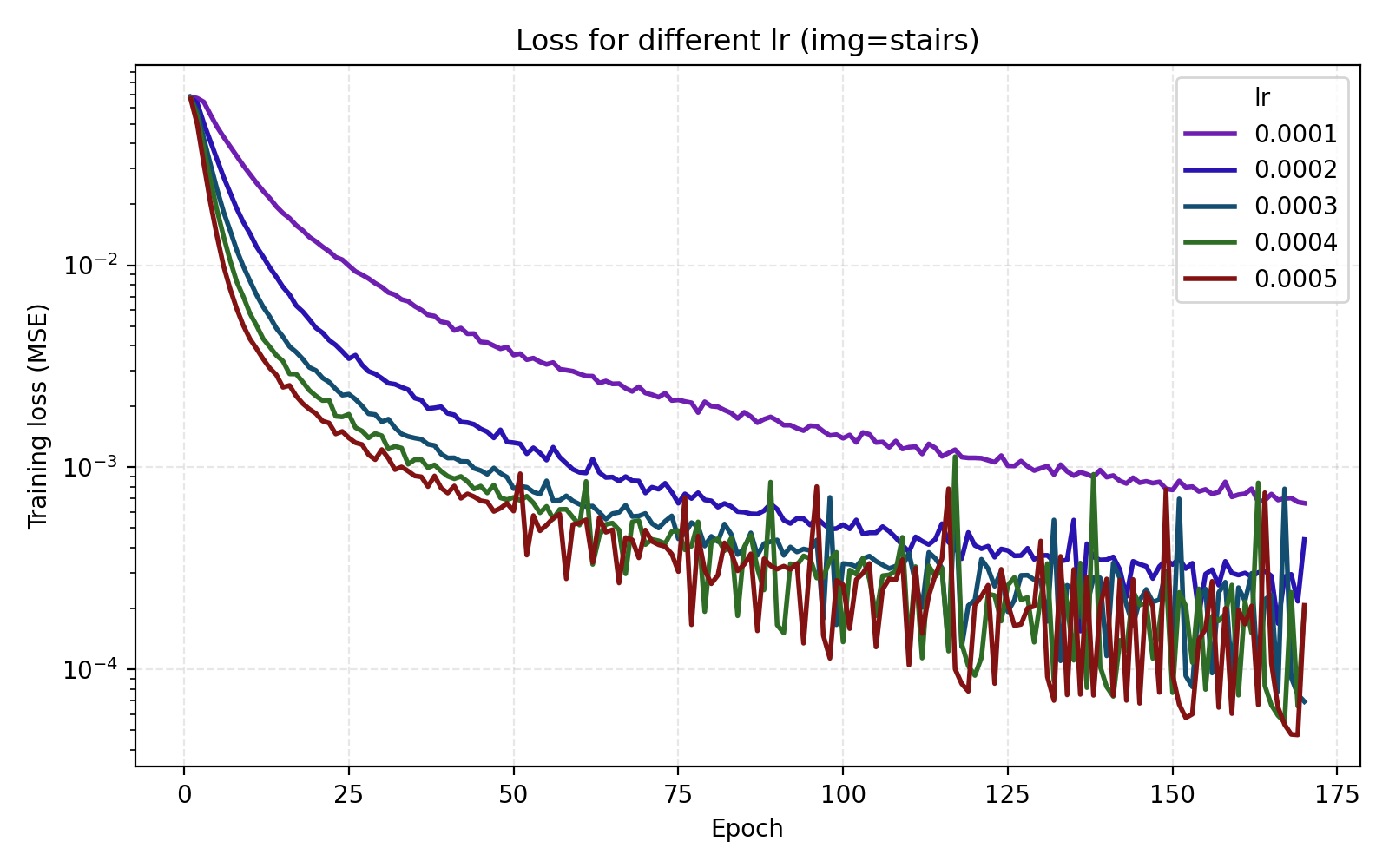
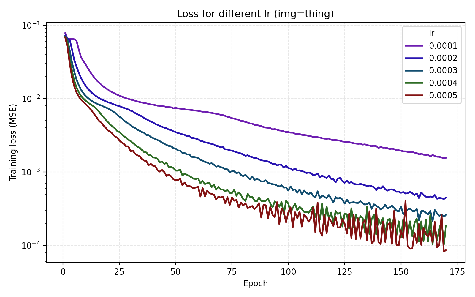
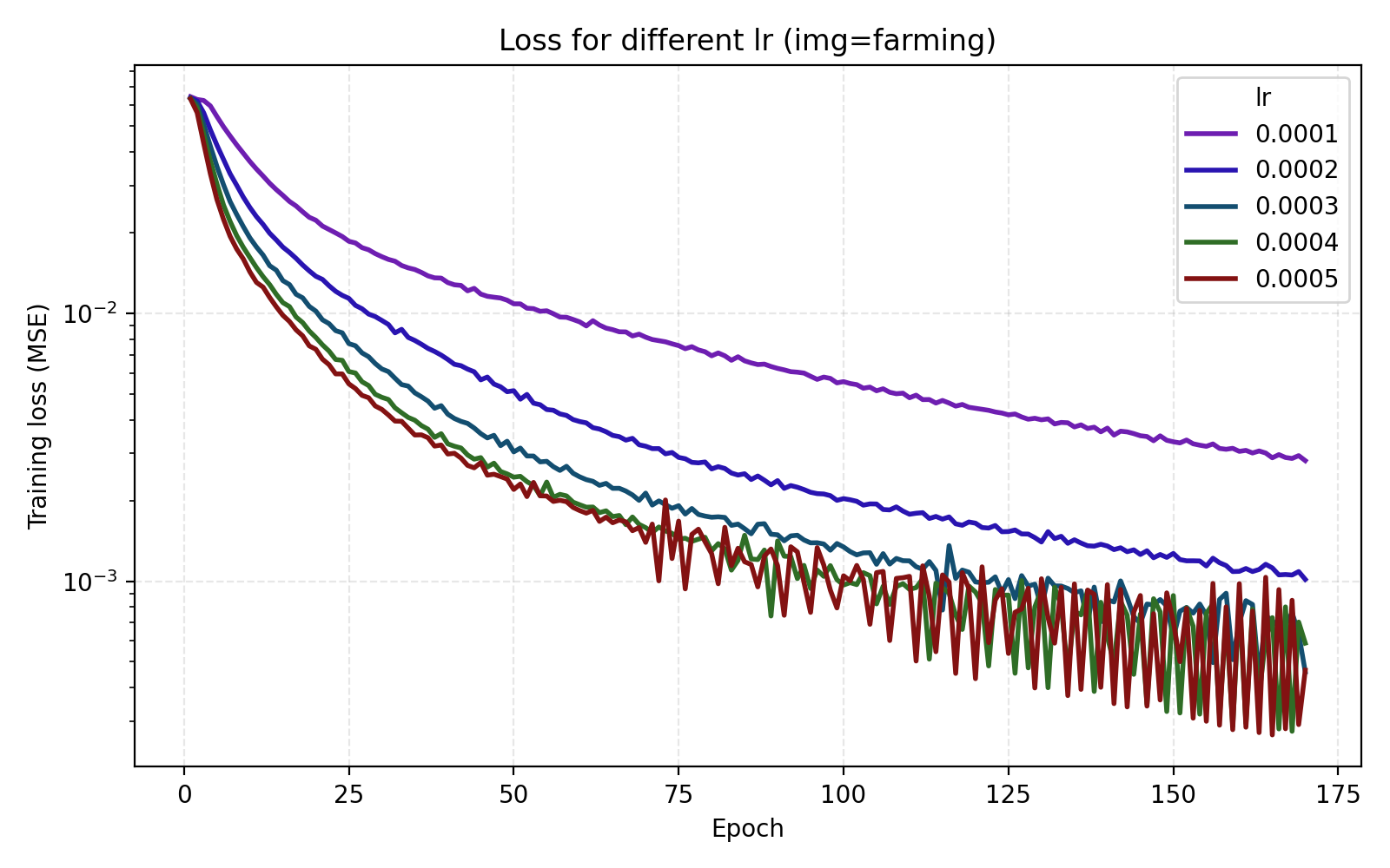
It is now easier to compare the five learning rates and we find that 5e-4 is optimal in this case.
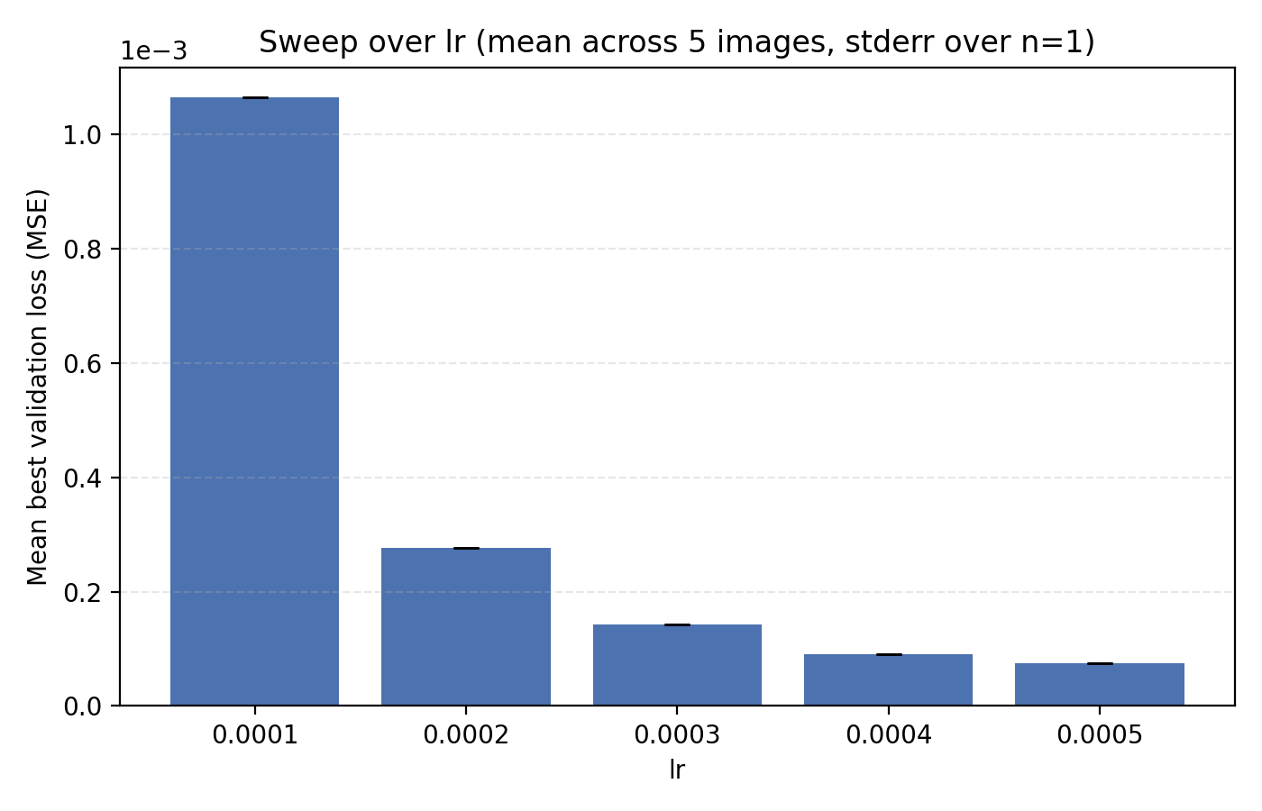
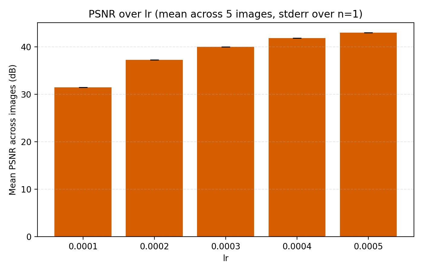
1e-4 to 5e-4.
Still, we choose to set lr = 4e-4 just for the additional stability since we see that higher learning rates lead to oscillations in the loss once it is low enough.
At this point, the PSNR is high enough that the images are almost perfectly captured by the INR. Below is a version of the training video from earlier with this model.
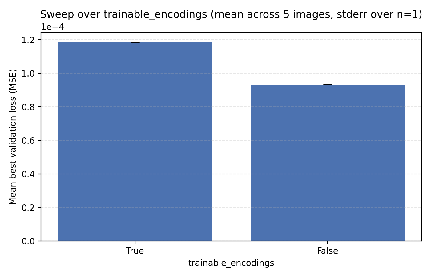
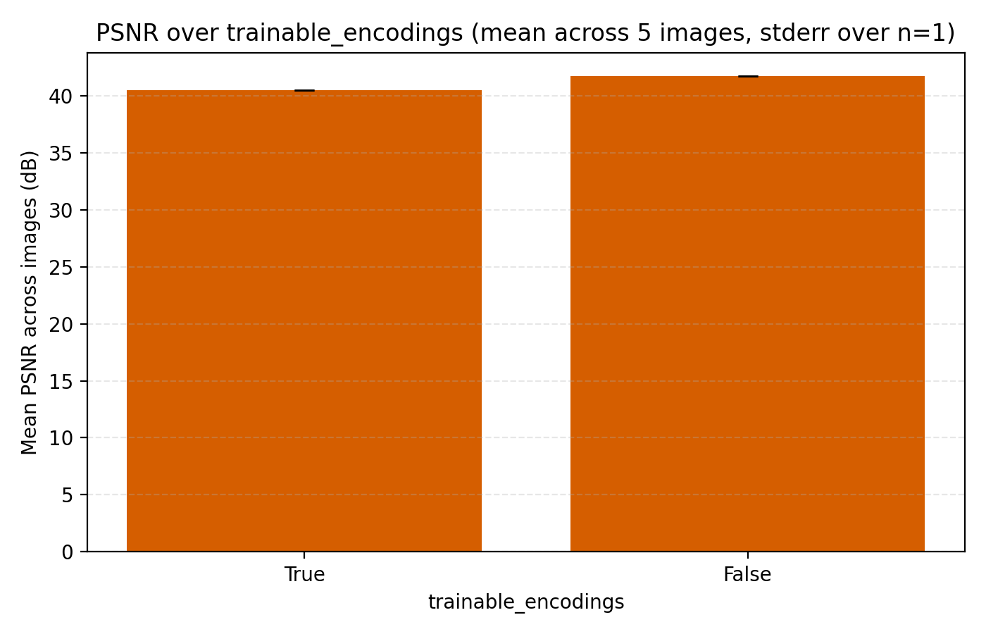
Next up we look at learnable frequencies. This means that we still initialize the frequencies in the positional encodings with standard deviation 80 but treat them as learnable model parameters. Here we see that trainable encodings do not improve performance.
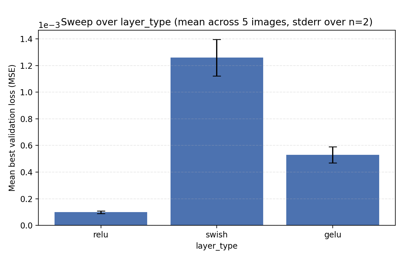
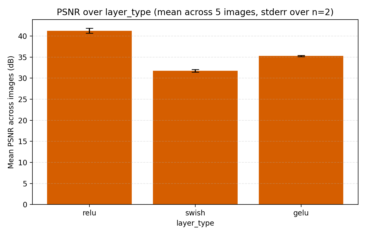
The final choice we look at is the activation function. Since we are using positional encodings, we are only comparing some standard choices, specifically ReLU, GELU and Swish. So far all our sweeping has been done with ReLU so it perhaps should not be a surprise that it performs best. Still, its margin is at least slightly remarkable.
The last property we look at is Gabor feature encodings. Just as for the activation function, we have so far made the (few) decisions about the architecture to optimize for Fourier features which puts Gabor features at a disadvantage. Since for Gabor features each dimension in encoding_dim has less energy since it is localized in position, we explore higher dimensional encoding dimensions at the same time.


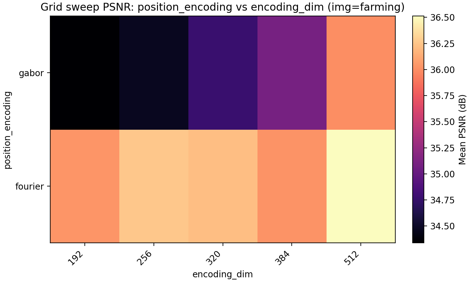
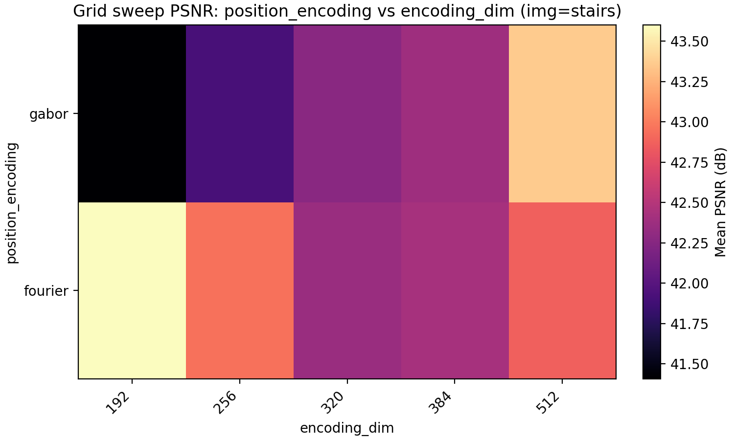

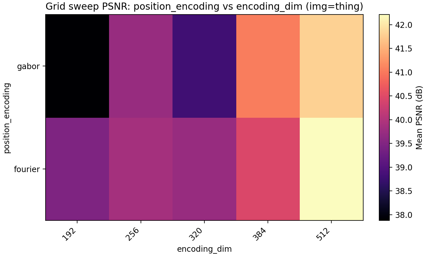
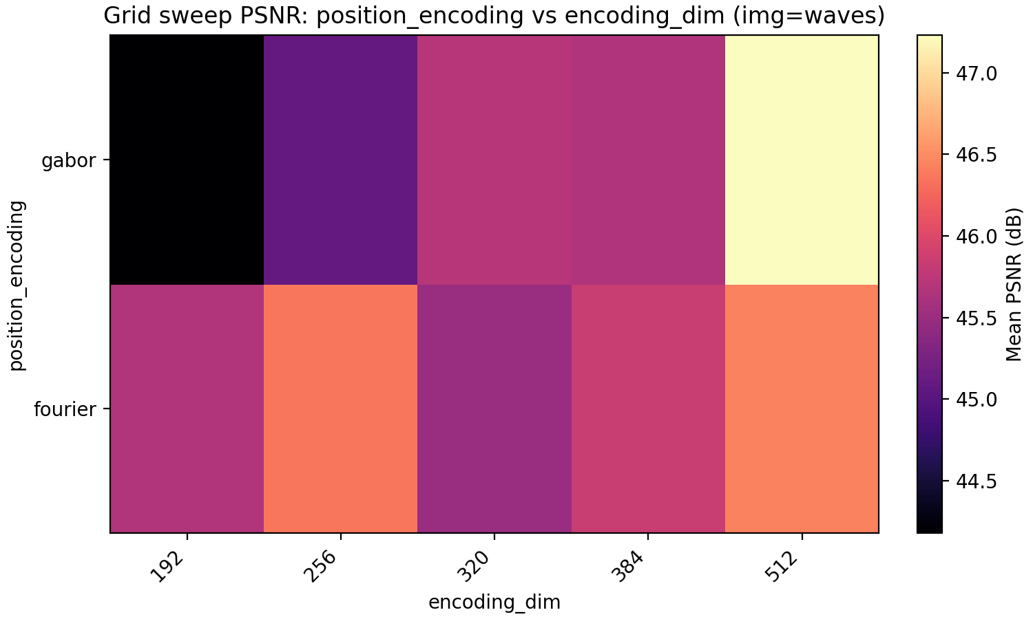
The result is very even with Gabor feature coming out on top for PSNR but not MSE but only at higher encoding dimension. Note meanwhile that the MSE and PSNR for Fourier features barely improve when going from 192 to 384 encoding dimensions. A conclusion that may be made is that Fourier features benefit less from larger encoding dimension but is preferable for a smaller model.
Gabor features have the additional effective hyperparameter deciding how to choose the widths of the Gabor atoms. In the code, we have set this to $0.1 \sqrt{\frac{d_{enc}}{256}}$ where $d_{enc}$ is the per-dimension encoding dimension so half of our actual encoding dimension in the 2D case. This choice was made to avoid an additional hyperparameter but would obviously benefit from tuning. Still, we stick with Gabor features for now.
Improving MLPs
We now turn to the three techniques of improving MLPs mentioned earlier, mixture-of-experts, LayerNorm and skip connections. LayerNorm generally has the effect of stabilizing gradient flow which is more important for deeper networks. With how we have pushed the model so far, it is thus conceivable that it should possibly help in this case. We find that it does so greatly.
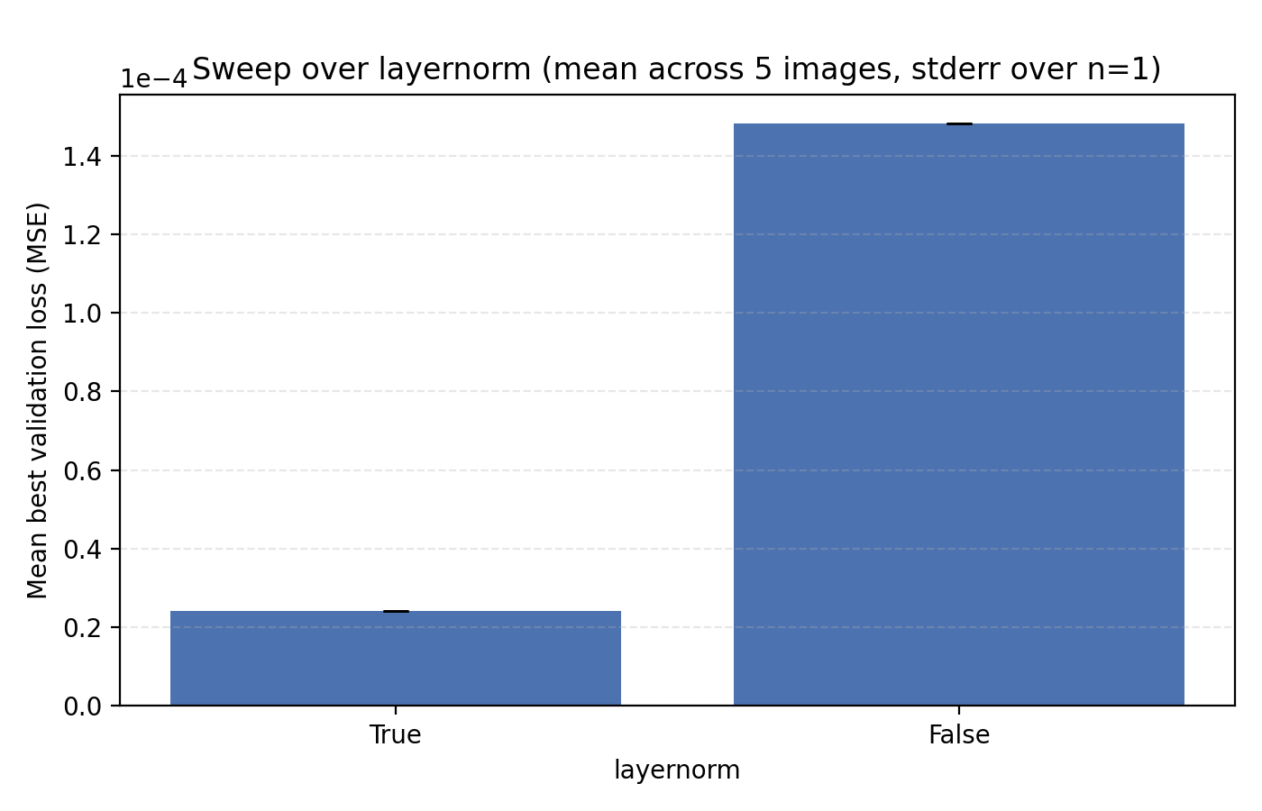
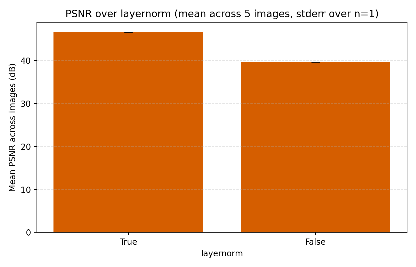
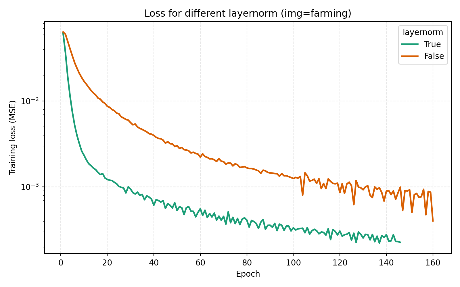
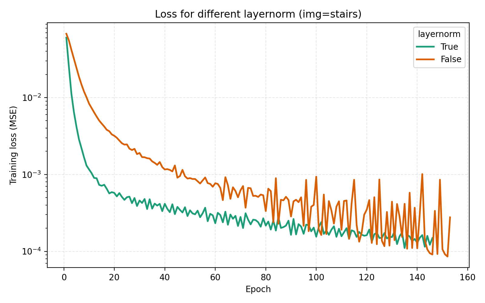
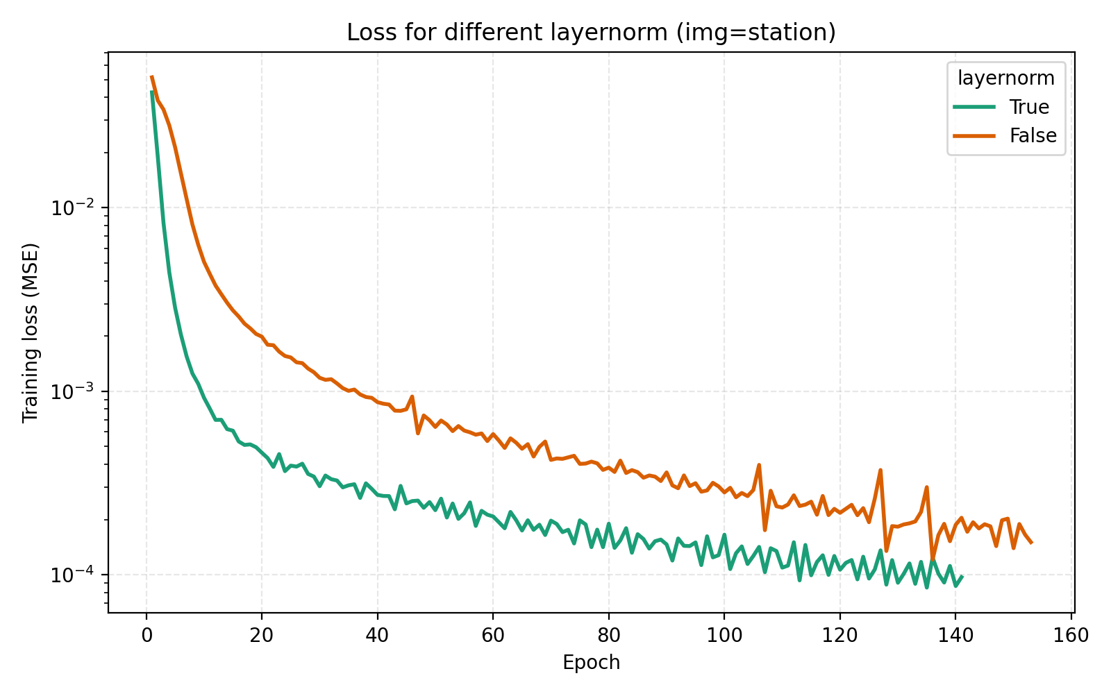
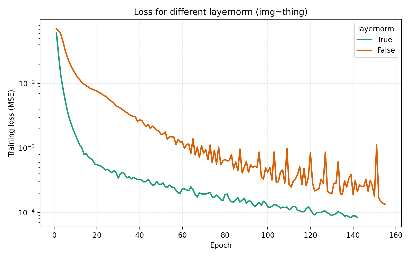
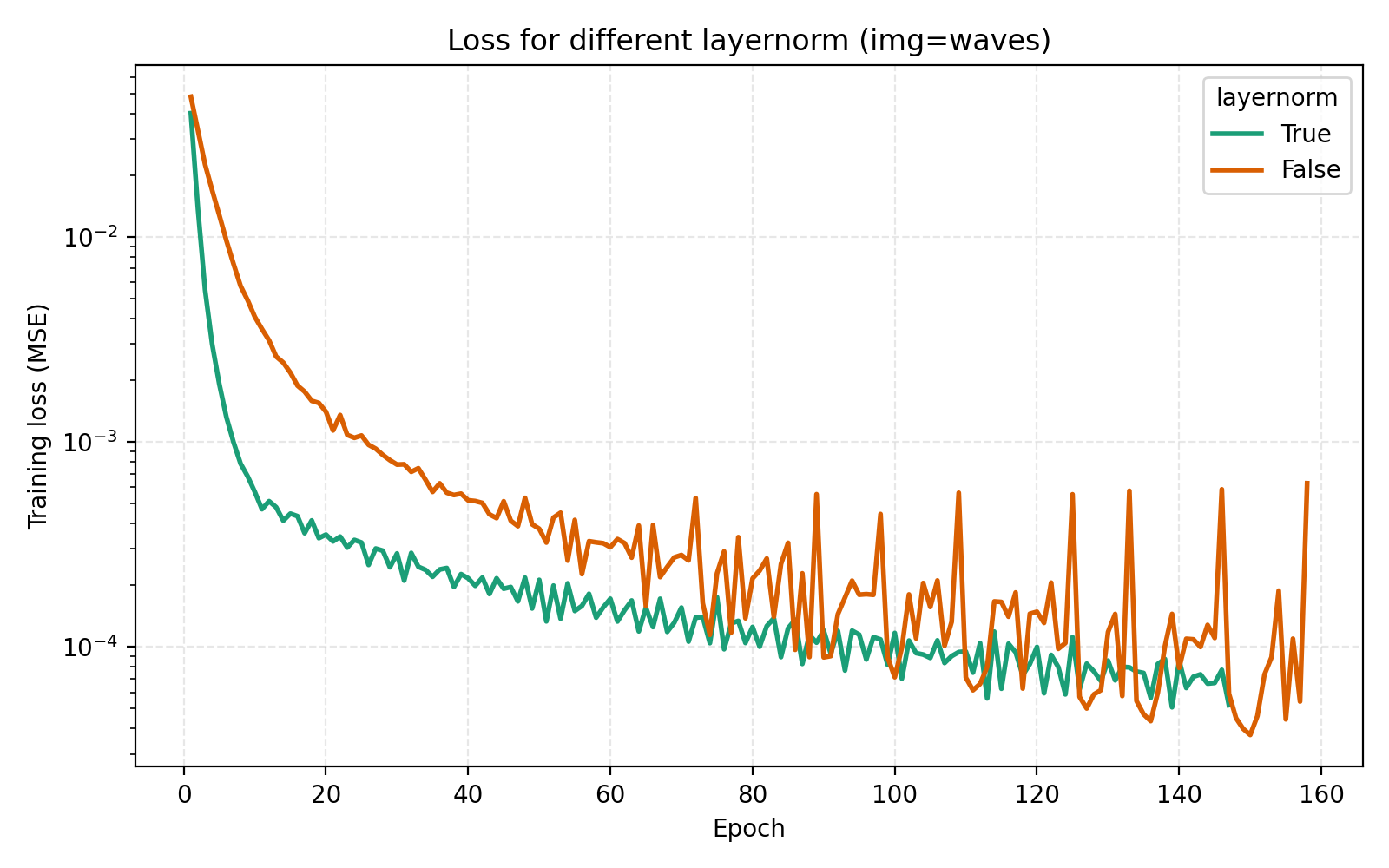
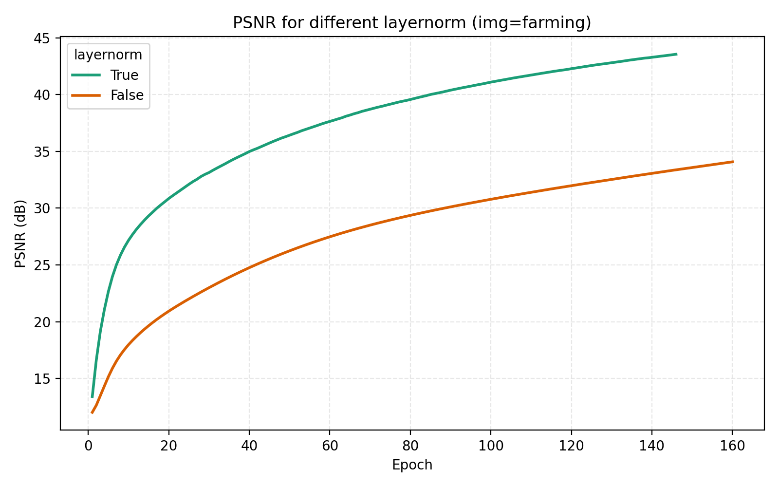
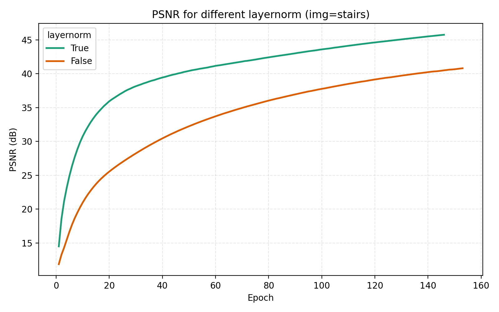
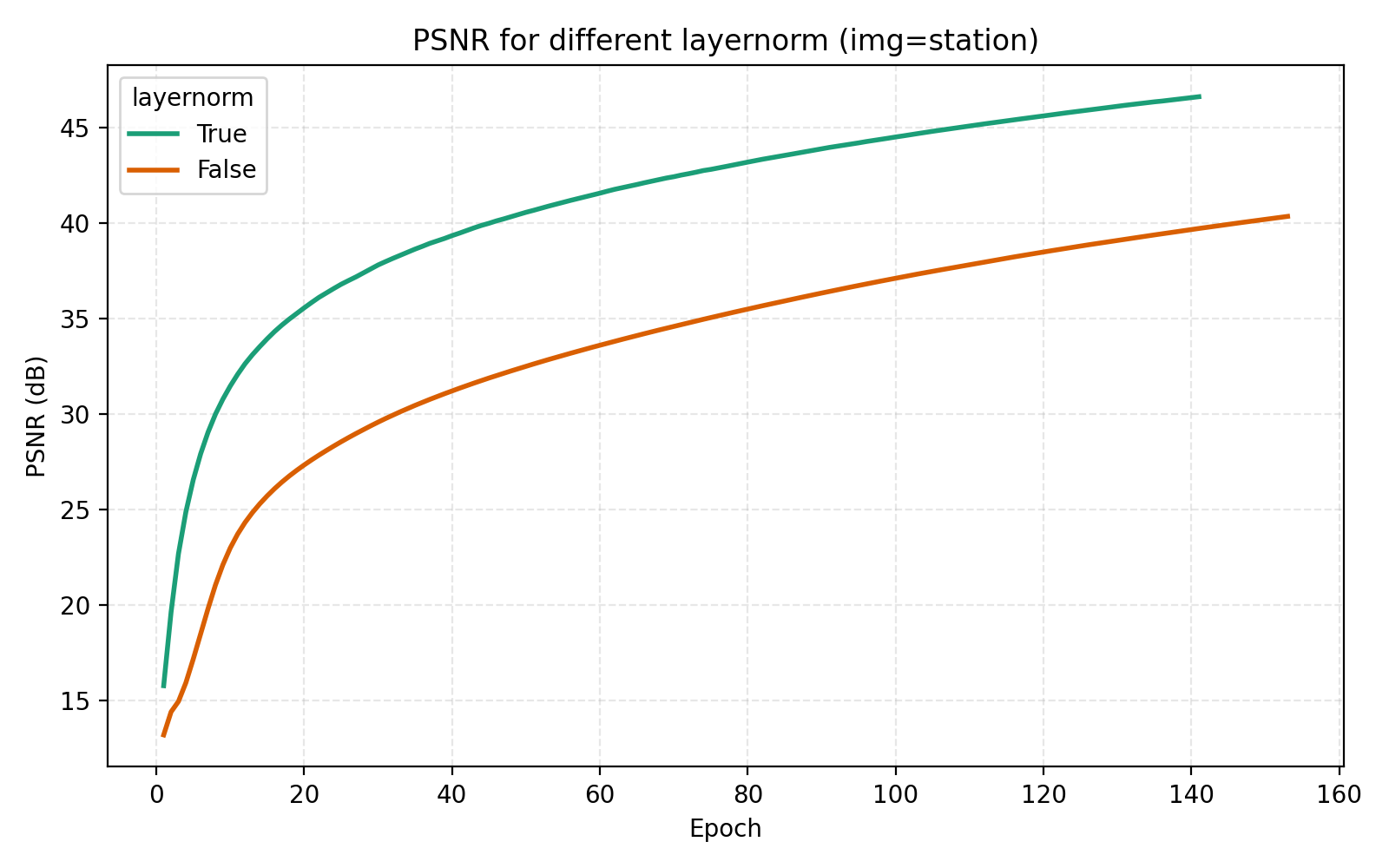
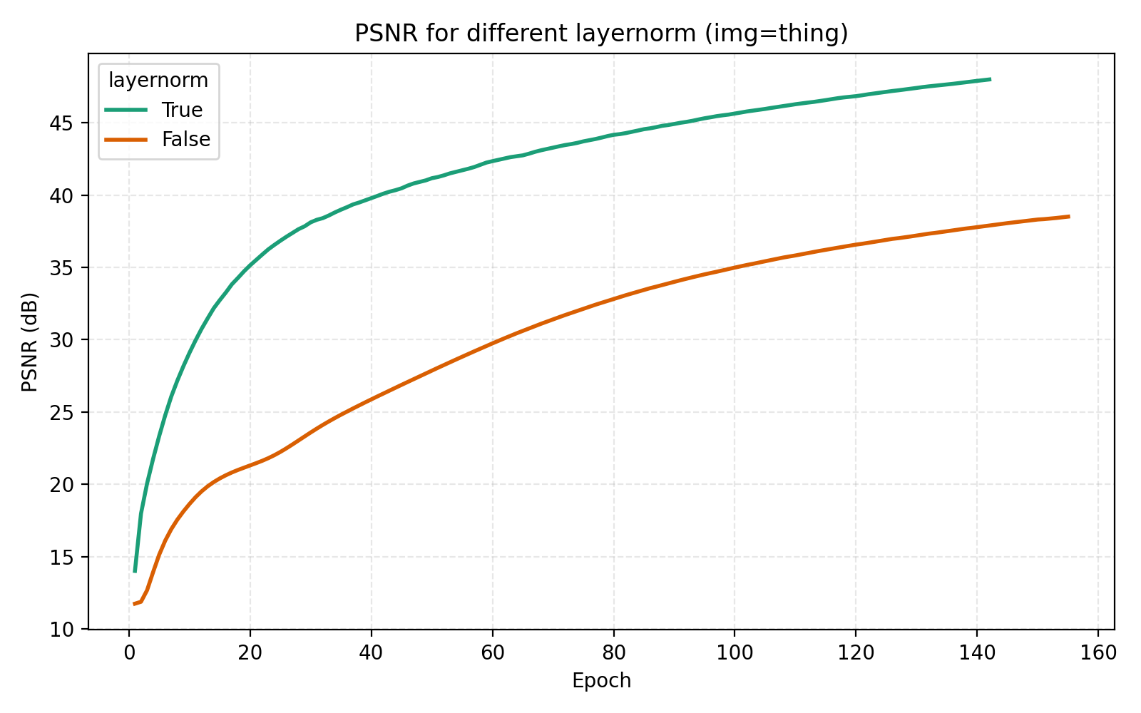
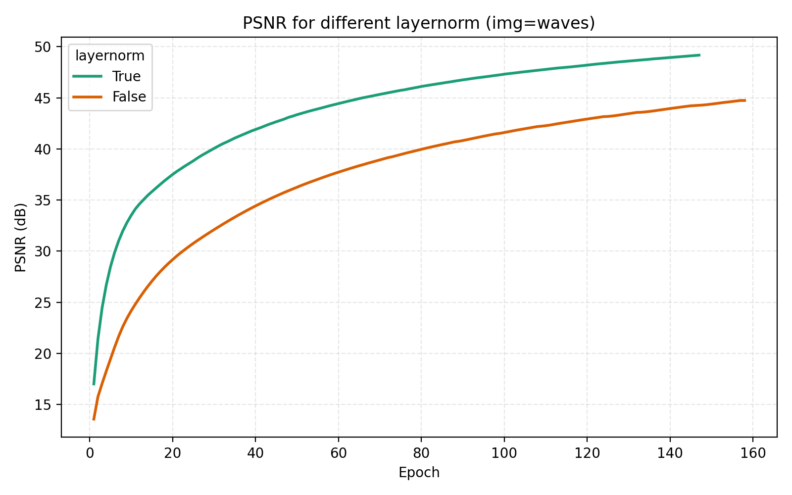
While this looks like a clear win for LayerNorm, if we look closer at the MSE for stairs (image #2) and waves (image #5), we see that MSE dips slightly lower at its best. However for PSNR the win for layernorm = True is clear and so we adopt it. Note also in the figures how much faster the network is when training with LayerNorm active. During the preparation of this post I also looked at RMSNorm and pre/post LayerNorm but found no big differences. This implementation is for post-LayerNorm.
Since LayerNorm has effectively given us a boost in performance, we turn to MoE to check if it is better spent on another copy of the network, more parameters, or keep spending the extra time training deeper. On a conceptual layer, MoEs for INRs are appealing since you could have different experts learn different parts of the image.
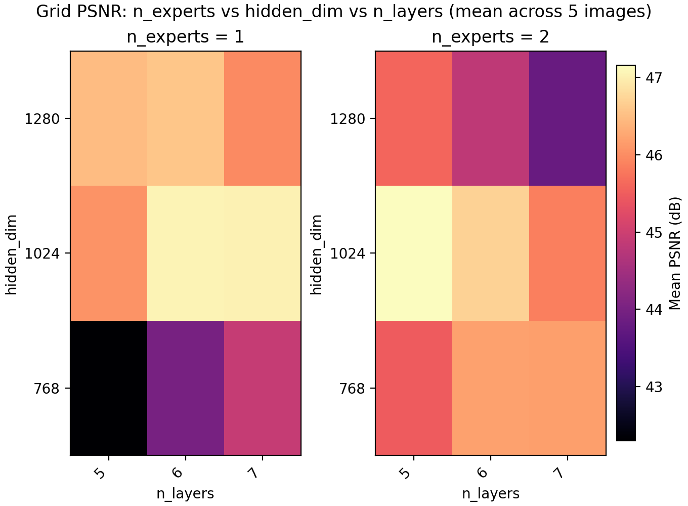
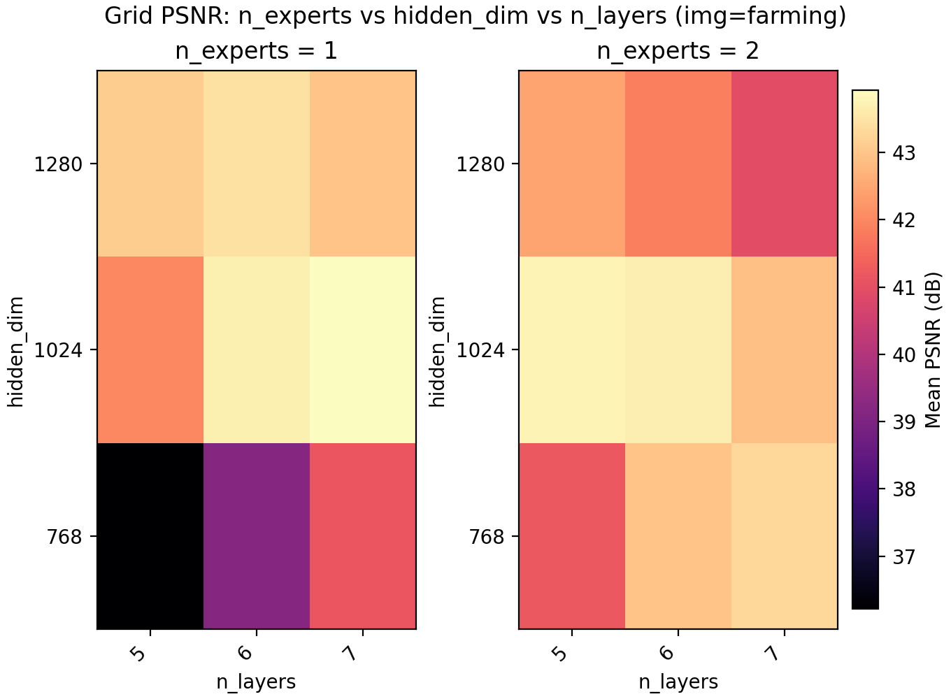
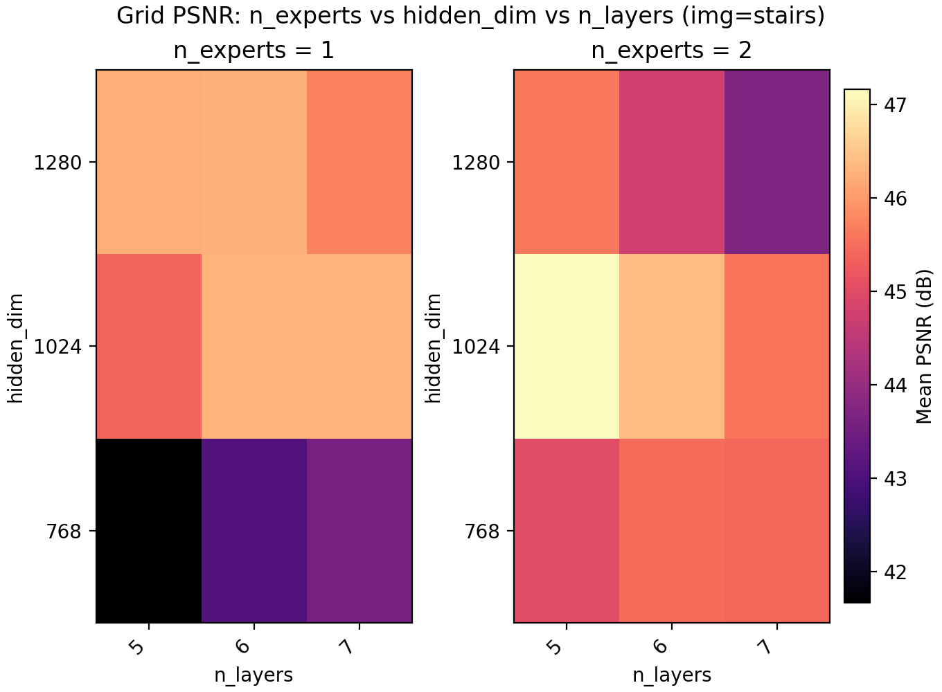
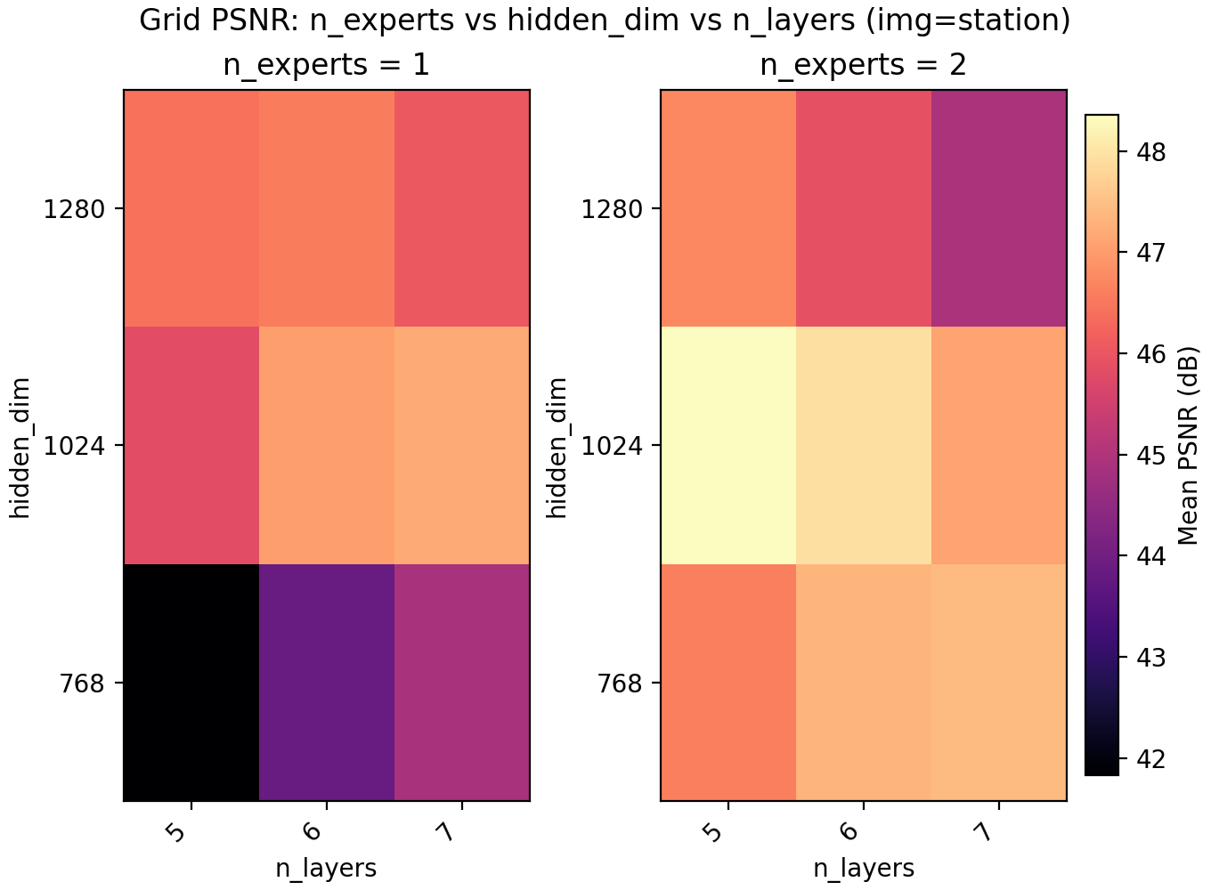
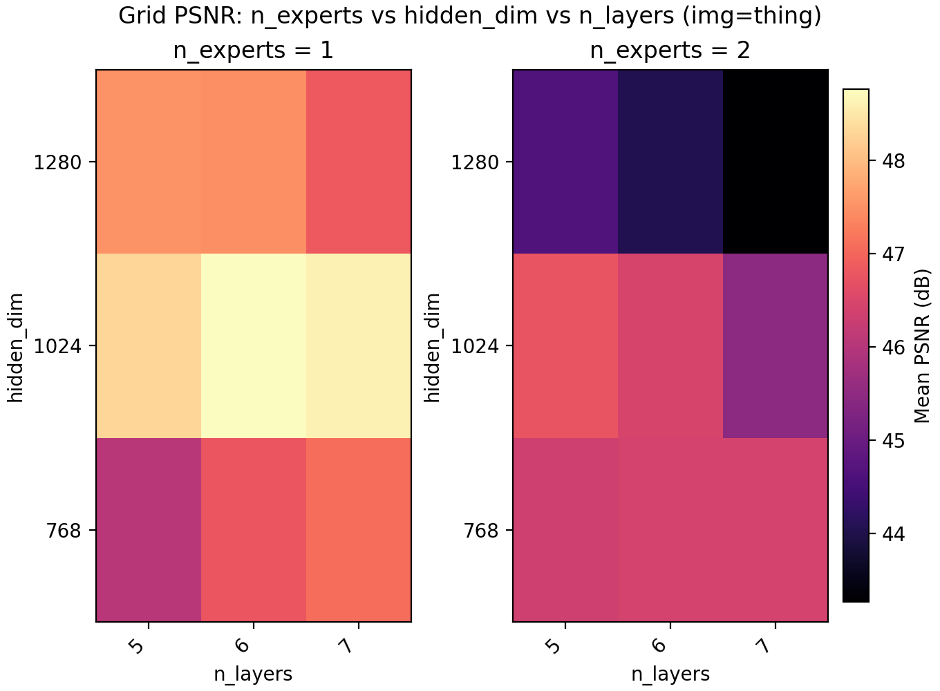
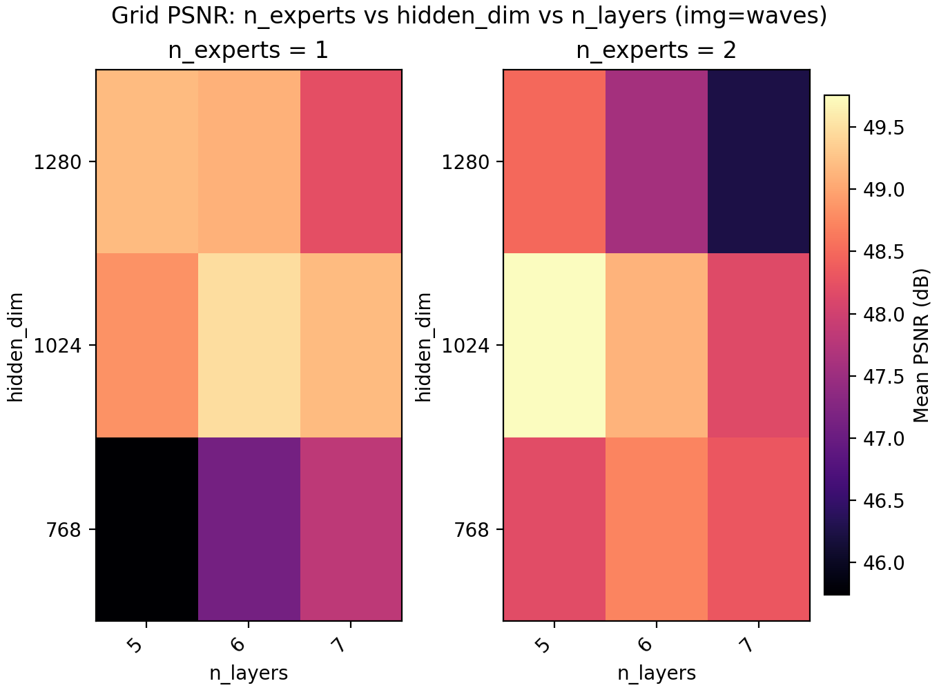
For the results we find a very slight edge for n_experts = 2 but at two training runs per configuration and image, the result is not statistically significant. Still, we keep it and lower n_layers to 5 to get a model with 6.8M parameters with a PSNR of 47.15.
Lastly skip connections turns out to have a small negative effect on performance, as well as slow down training slightly due to the increased computational load. It is possible skip connections do not become important until the networks are much deeper.
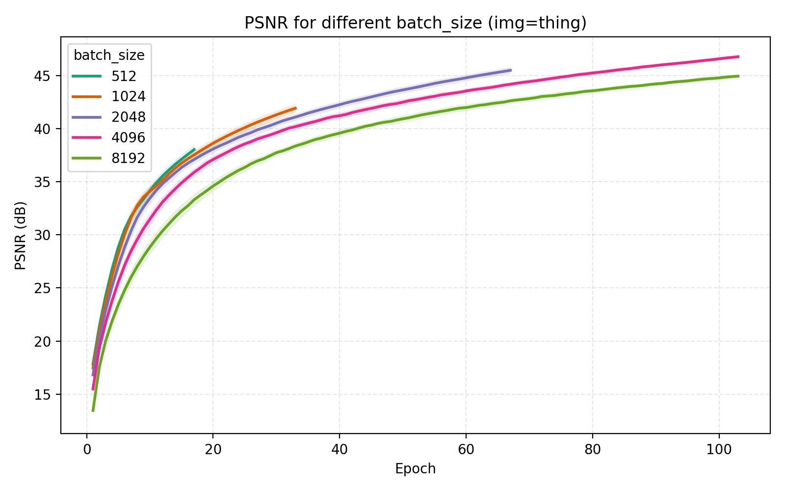
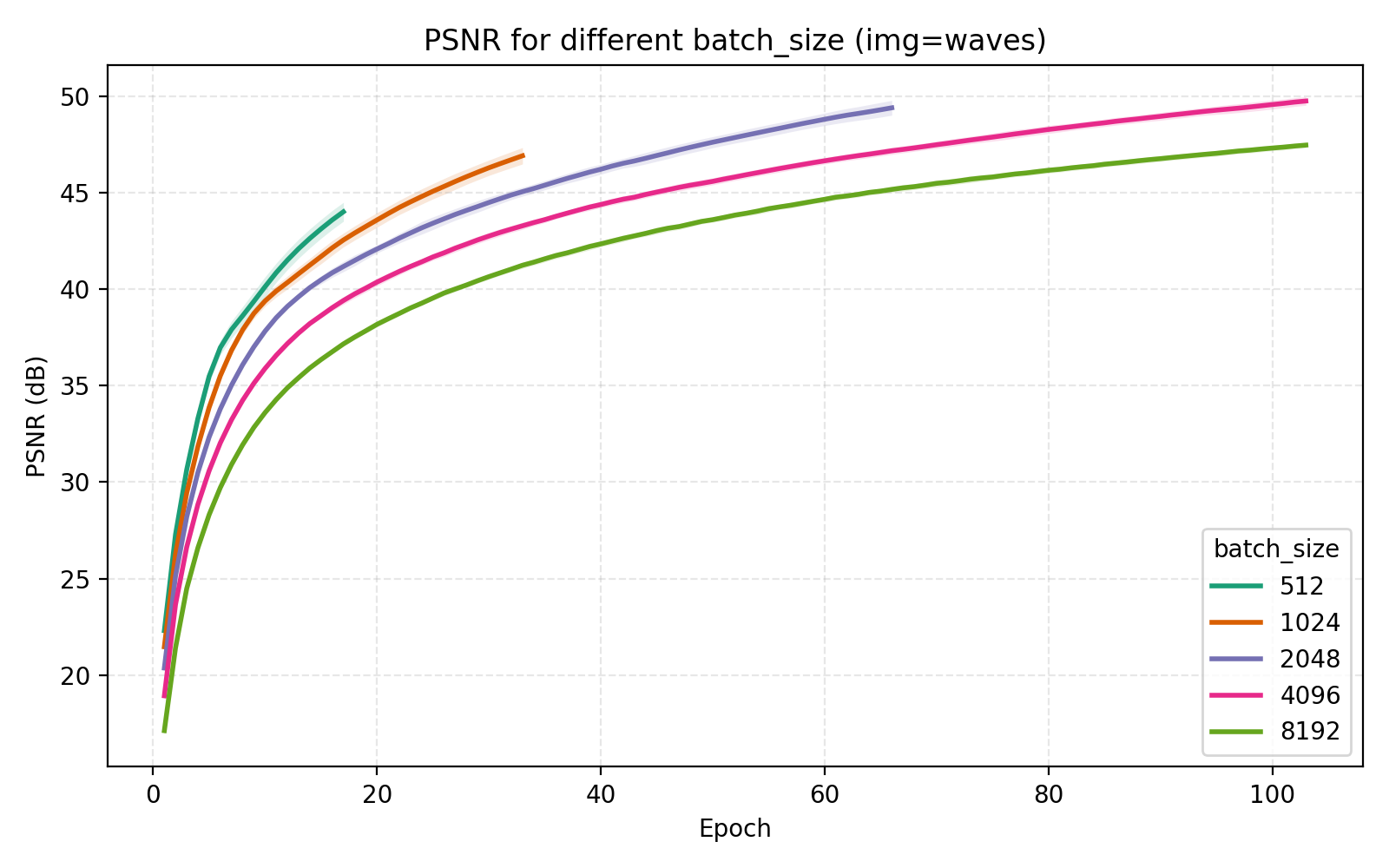
At this point, with a PSNR at 47.15, the images are essentially perfectly captured by the networks. To some degree, this is the point of this post - by properly tweaking the architecture we can get a standard Fourier features MLP to have perfect performance with only three minutes of training on a modern GPU. Looking at the snapshots, even after only 5 epochs at a batch size of 4096 = 768×768 × 0.7%, the image is mostly learnt.
47.15. Put video in fullscreen to see details better.
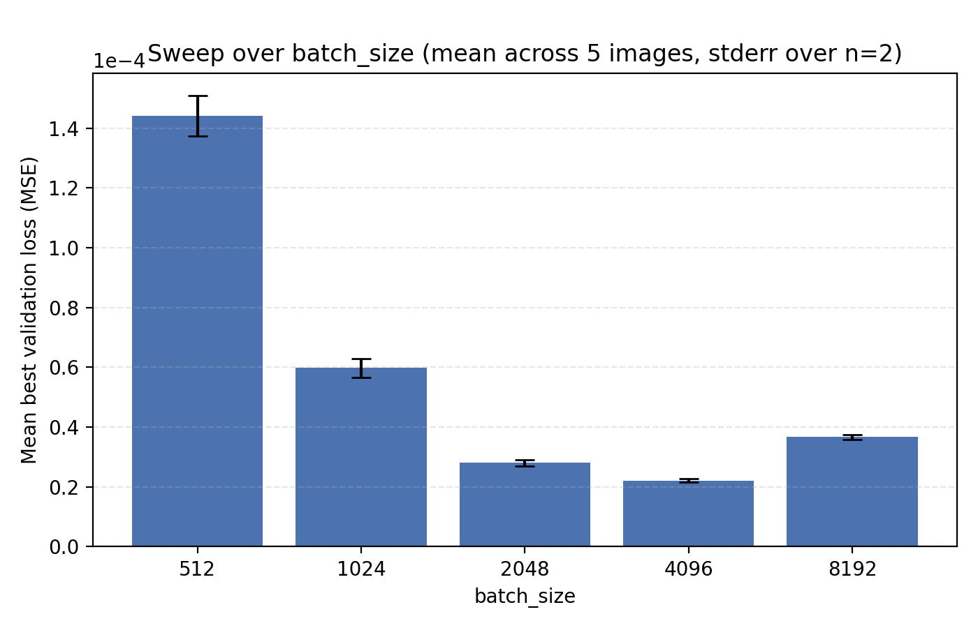
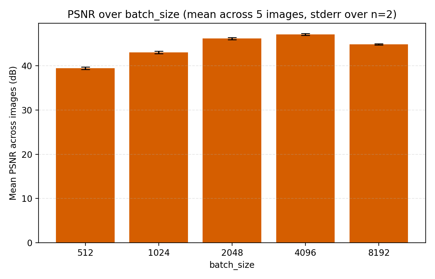
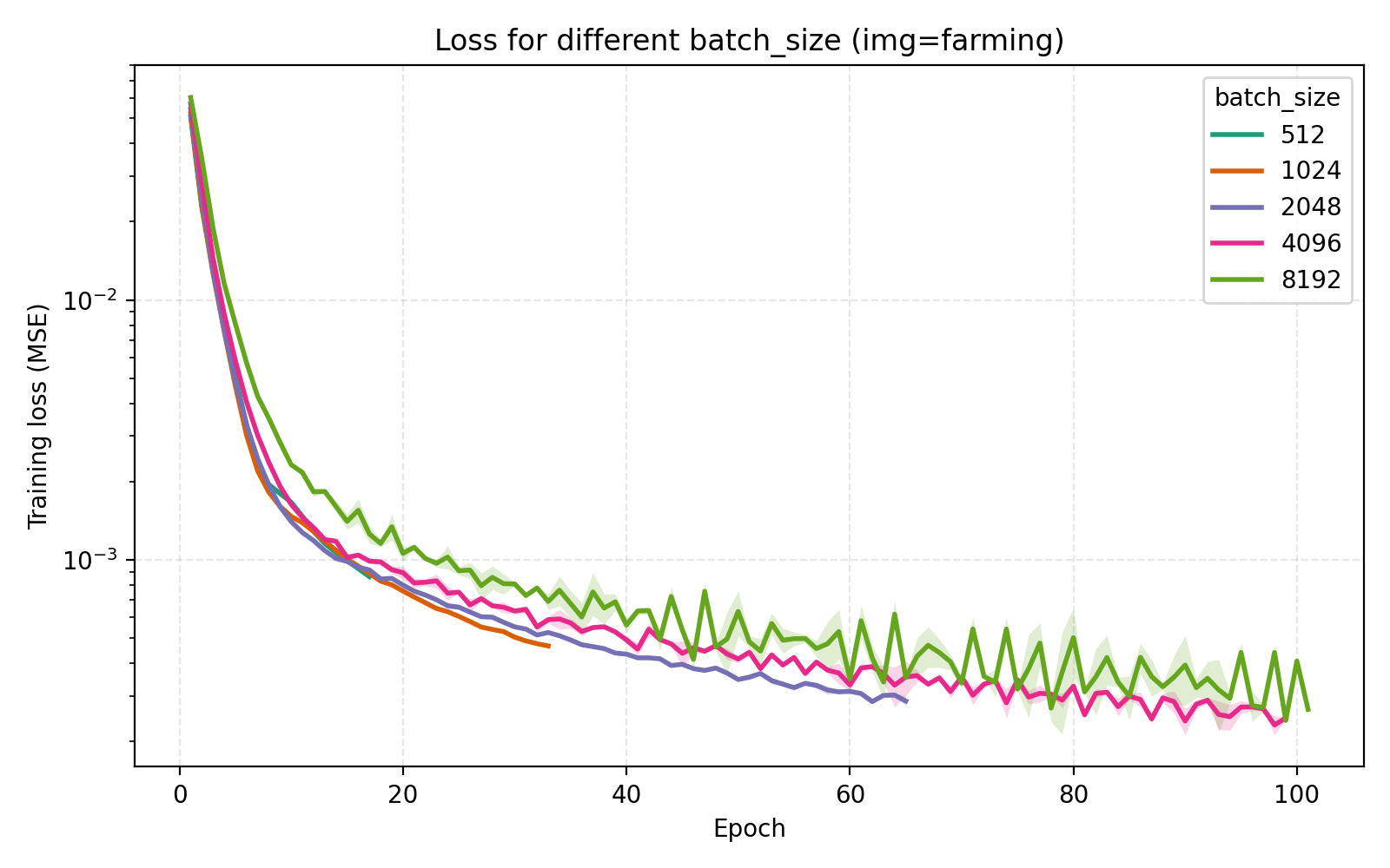
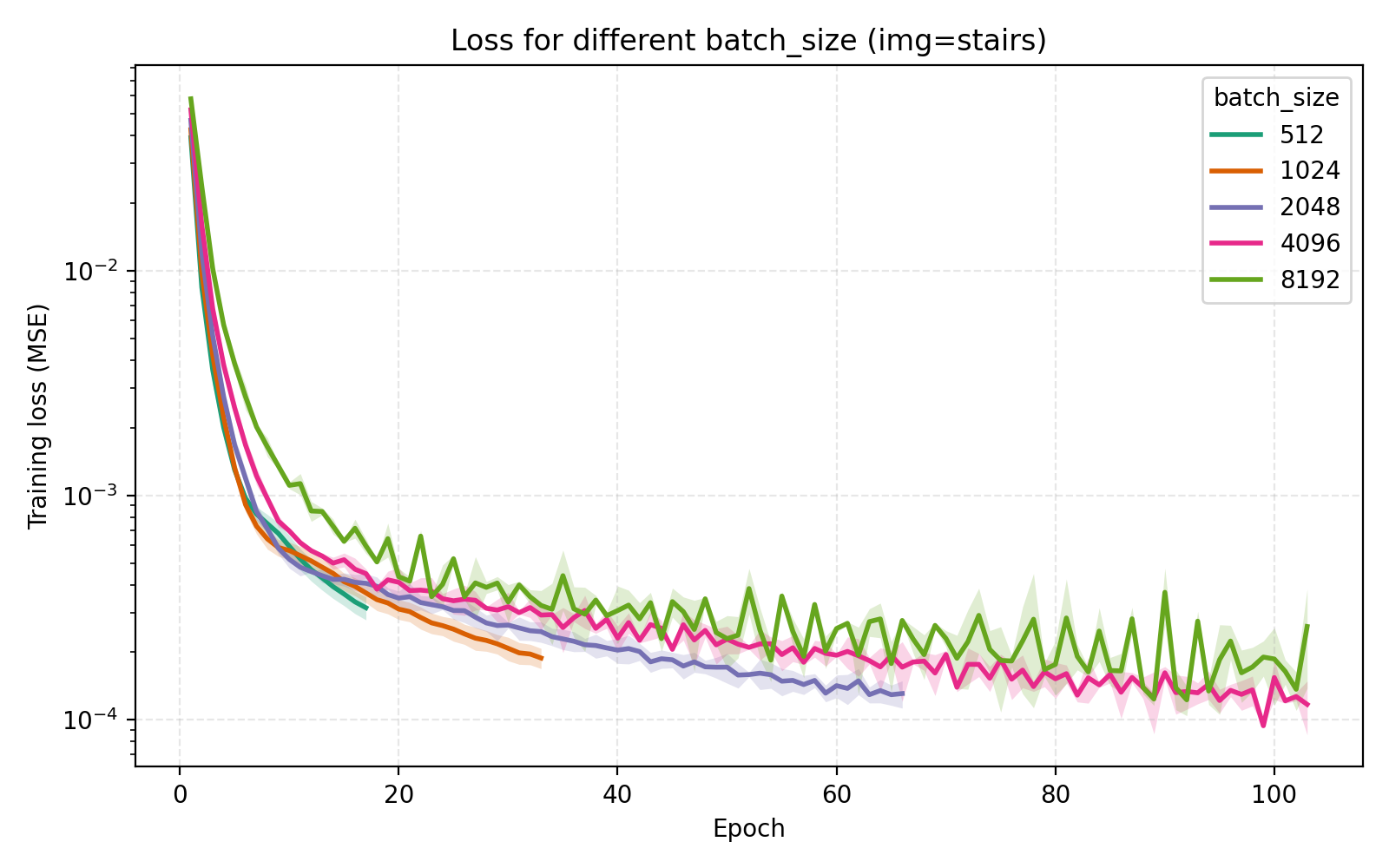
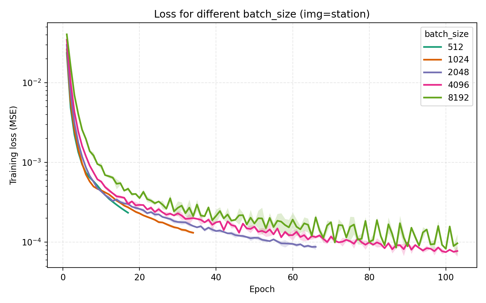
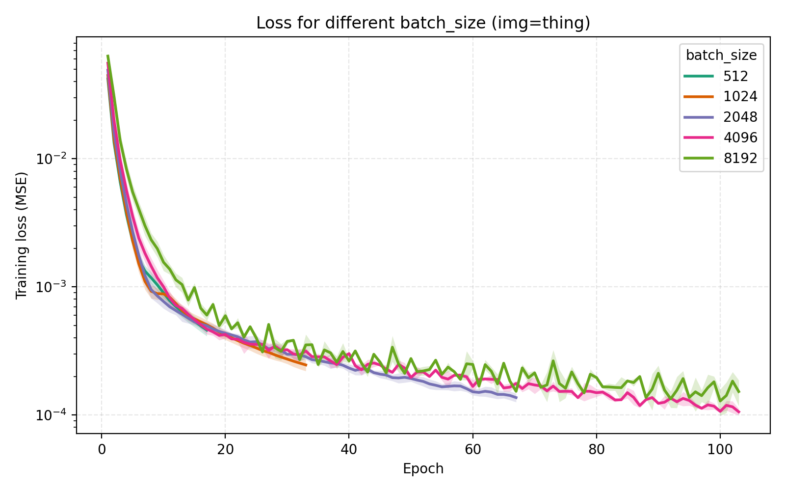
On the topic of batch_size, our choice of 4096 is indeed optimal among the canonical $2^n$ alternatives.
Concluding remarks
In the process of tweaking all the available hyperparameters, we have essentially saturated our benchmark problem. There are two main implications of this worth mentioning:
- The benchmark problem might have been too easy If we really want to push architectures to their limits, we should place a lower time limit or possibly added a memory limit.
- When comparing INR architectures, tweaking all variables are very important To some degree, this is an impossible ask. Benchmarks generally fix a lot of parameters and only change one thing. The point of this post is to show that even a simple architecture can be pushed very far with a limited compute budget.
Generally, the goal of INRs is not to simply learn a function but to be used for some downstream task involving reconstruction from partial measurements such as superresolution, CT reconstruction or novel view synthesis. These are more appropriate benchmarks but at the same time less general.
The usage of LayerNorm in the MLP is perhaps the most important step we took in the optimization procedure. The effectiveness of LayerNorm has been noticed elsewhere (e.g., INCODE, SL²A-INR, among others) but is still important to push.