What do learned positional embeddings look like?
By Simon Halvdansson | Nov. 2025
Transformer blocks are famously permutation equivariant, meaning that without intervention, they cannot tell the order of the tokens. One solution to this problem is to learn a tensor of shape (d_model, seq_len) which we add after embedding our data. It is not clear a priori what properties these learned positional embeddings should take and it turns out they are substantially different from classical sinusoidal positional embeddings. In this post, we give some background on positional embeddings and investigate what they look like from different directions.
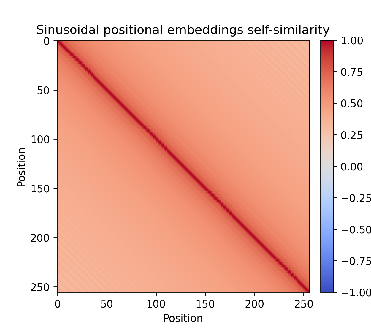
Figure: Cosine self-similarity of learned positional embeddings for
seq_len = 256 (left) and standard sinusoidal positional embeddings (right).
We will first go over some of the mathematics behind positional embeddings before looking closer at visualizations.
Mathematics of additive positional embeddings
The self-attention mechanism is a self-map which is equivariant to permutations, meaning that if we permute the inputs, the output is permuted in the same way. To see this formally, let $P$ be a permutation matrix and consider
$$
\begin{align*}
\operatorname{attention}(PX) &= \operatorname{softmax}\left( \frac{P X W_Q ( P X W_K)^T}{\sqrt{d_k}} \right) PX W_V\\ &= P \operatorname{softmax}\left( \frac{X W_Q ( X W_K)^T}{\sqrt{d_k}} \right) P^T PX W_V = P \operatorname{attention}(X).
\end{align*}
$$
When we extract a value from the transformer after the final transformer block, we usually read a special [CLS] token or pool all the tokens. Either way, this does not let the transformer react to the order of the tokens in any special way. The original transformer paper used sinusoidal positional embeddings meaning that each token got added a fixed vector which was a sampled sinusoid with increasing frequency along the token dimension. This breaks permutation invariance by adding three new terms to the query-key multiplication in a way which depends on the position. Specifically, with $X$ replaced by $X + E_{\text{emb}}$,
$$
\begin{align*}
\operatorname{attention}(X) = \operatorname{softmax}\Bigg( &\frac{X W_Q (X W_K)^T}{\sqrt{d_k}} + \frac{X W_Q (E_{\text{emb}} W_K)^T}{\sqrt{d_k}} \\
&+ \frac{E_{\text{emb}} W_Q (X W_K)^T}{\sqrt{d_k}} + \frac{E_{\text{emb}} W_Q (E_{\text{emb}} W_K)^T}{\sqrt{d_k}} \Bigg) X W_V.
\end{align*}
$$
The output of the softmax, the attention weights, is a seq_len $\times$ seq_len matrix which we take to encode how much the new representation after the self-attention should be influenced by the other tokens. Indeed, $(A V)_i = \sum_{j=1}^L A_{ij} V_j$ where $L$ is seq_len. If this matrix is just the identity, this means that the new representations do not get any extra inter-token dependencies from the self attention (note that $V$ is already a function of $X$ so some inter-token dependency comes built in).
In the expanded form of the attention above, the first term in the softmax is just the standard attention scores. Meanwhile the second and third terms can be interpreted as their own query-key interactions where we somehow relate the positional embeddings to the content of the tokens (although the usefulness of these interactions are somewhat dubious). The last one is most interesting. If $W_Q W_K^T = I$, then the numerator is precisely the Gram matrix $E_\text{emb} E_{\text{emb}}^T$ which is essentially the cosine similarity from the first figure! Now since $W_Q W_K^T \neq I$, we don't get precisely this but rather something related to it. This provides at least some of the motivation for why we want a slow off diagonal decay of the self-similarity matrix; representation should be influenced more by tokens close by.
Newer ideas in positional embeddings generally treat the problem in a more direct way. A family of ideas going under the name relative positional embeddings have proposed changing the $QK^T$ multiplication in various ways, including replacing $E_{\text{emb}} W_Q W_K^T E_{\text{emb}}^T$ by $E_{\text{emb}} U U^T E_{\text{emb}}^T$ with the new matrix $U$ disentangled from the standard query and key projections. One can also directly add an $L \times L$ bias matrix $B$ to the attention scores. We will not look any further at these approaches here but refer to the review in the RoPE paper.
Embedding visualizations
So far, everything we have said about positional embeddings has been mostly speculation. Meanwhile, transformers and modern machine learning at large is firmly an empirical science. To actually investigate learned embedding, we train a simple 89M parameter LLM with n_layers=12, d_model=512 and n_head=4 on the TinyStories dataset. For more on the model, see the earlier post. Throughout training, we can take snapshots to see how the embeddings evolve.
The perhaps most obvious, but also most crude, way to visualize learned embeddings are by plotting the seq_len$\times$d_model matrix which we learn. This is done in the figure below:
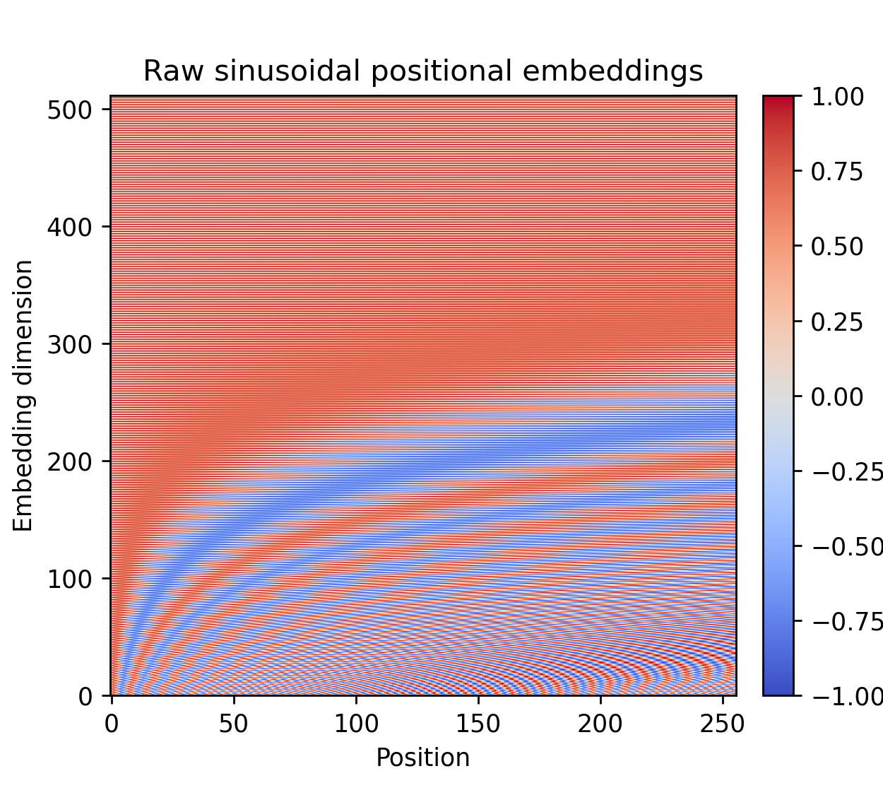
Figure: Positional embedding matrix over 2 epochs of training, learned on the left and sinusoidal on the right.
In the figure we see some structure evolve for the learned positional embeddings, at least along the position axis in the form of horizontal lines. This means that for two positions near each other, there appears to be a correlation in the values for a certain given dimension, often at least. Meanwhile along a specific position, there is not any apparent correlation as we traverse the embedding dimension. This makes sense because there is no a priori reason that hidden dimension #33 should have anything to do with hidden dimension #34. Next up we look closer at three dimensions specific embeddings.
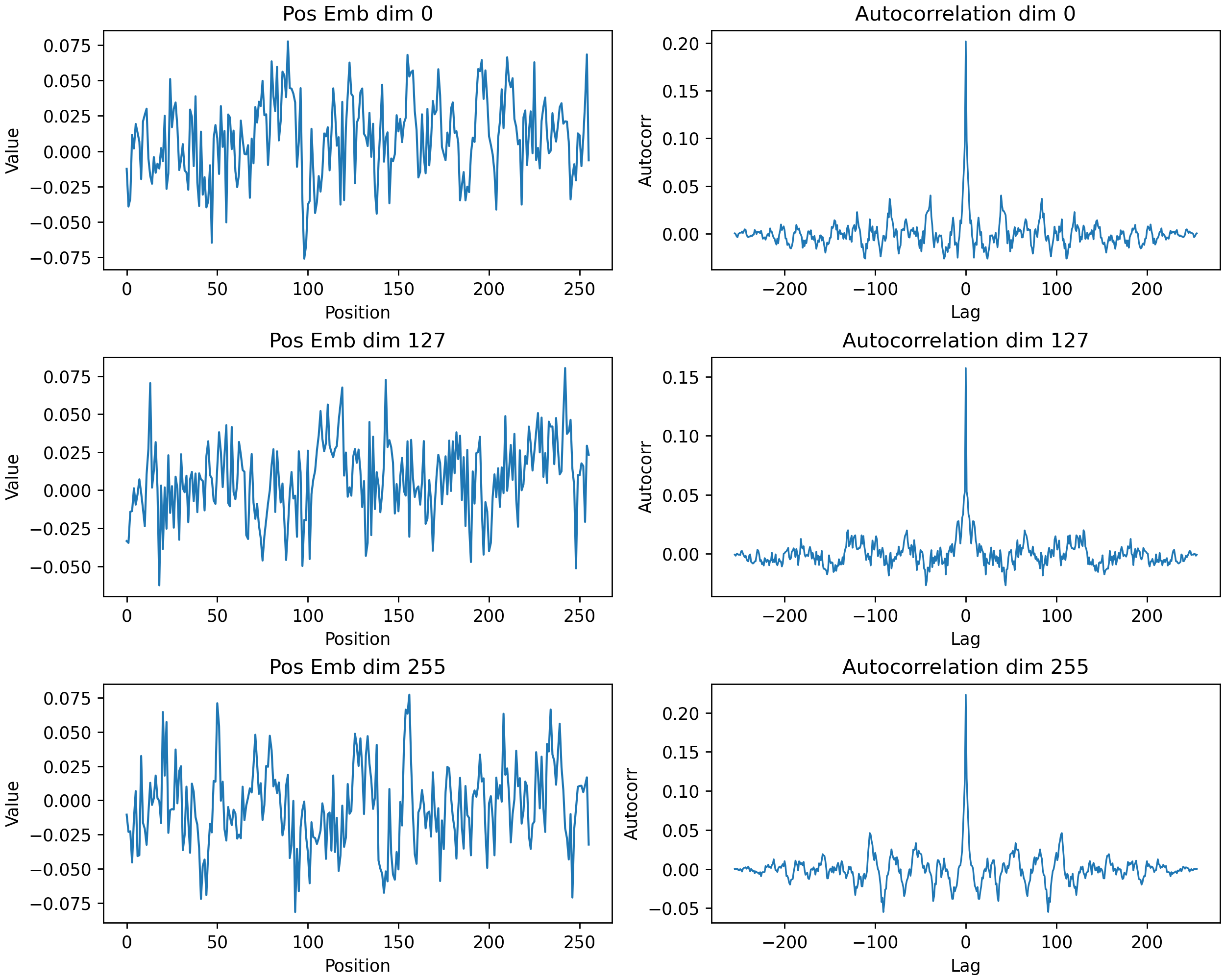
Figure: Learned positional embeddings along the position axis, and their Fourier transforms.
From the images, it is somewhat hard to determine if there is any drift or autocorrelation. One way to investigate it is to look at the mean of the absolute values of the autocorrelations, taken over the different embedding dimensions.
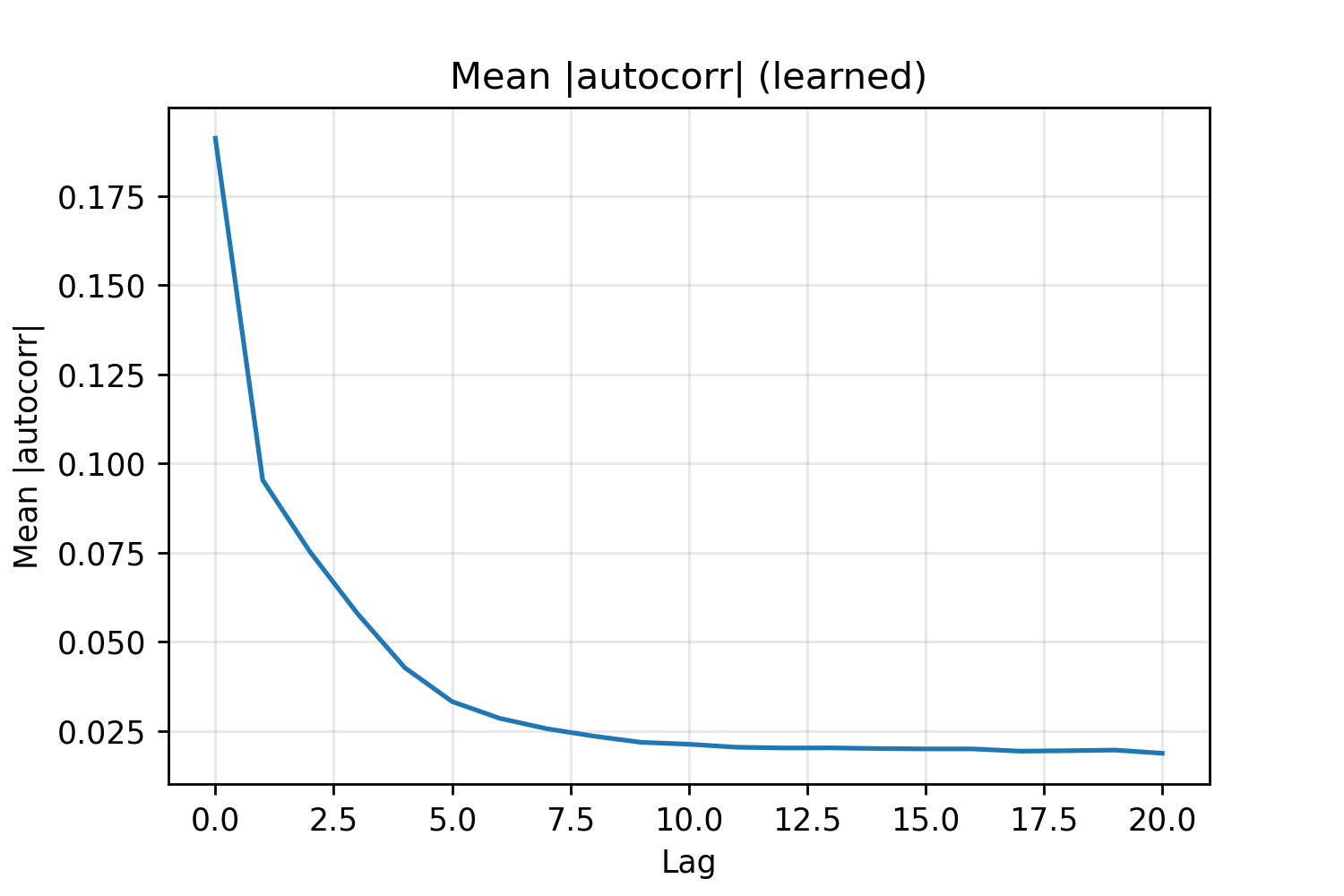
Figure: Mean over all embedding dimensions of the autocorrelation for lag 0 to 20.
In this form, the autocorrelation is obvious and we can conclude that there is continuity along the position axis. This makes sense because positions near each other should look similar to the model. If we compare this to sinusoidal positional embeddings, the difference is stark and the patterns are much smoother.
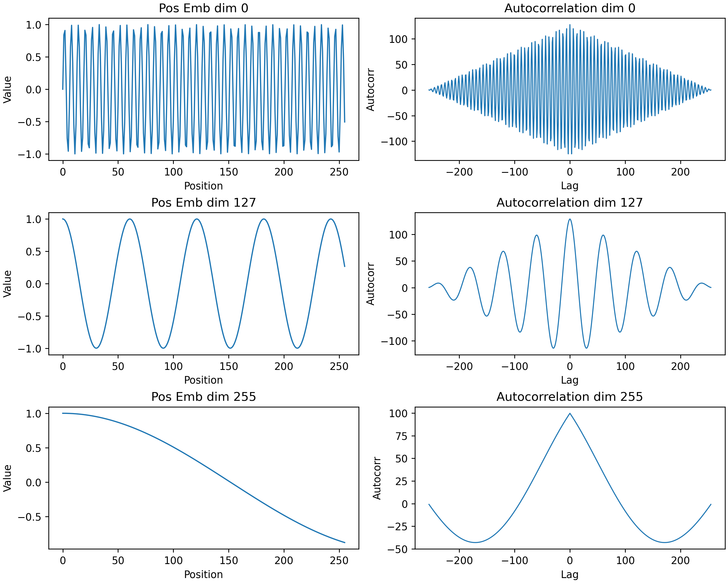
Figure: Sinusoidal positional embeddings along the position axis, and their Fourier transforms.
The mean of the absolute value of the autocorrelation has a similar decay to those of the learned embedding, albeit with a slower decay. Inspired by the $E_{\text{emb}} W_Q W_K^T E_{\text{emb}}^T$ term discussed earlier, we turn to look at the inner products of embeddings.
Cosine self-similarity
Self-similarity is a common way to visualize the inter-dependence between positional embeddings and is the method we used for the figure at the top of the post, and below. Formally, the cosine self-similarity between two vectors $u,v$ is the normalized inner product
$$
\frac{\langle u,v\rangle}{ \Vert u \Vert \Vert v \Vert}
$$
which we know is always normalized in the $[-1, 1]$ range. In the figure, we see how the off-diagonal decay gets weaker as the embeddings settle in.
Figure: Cosine self-similarity of learned positional embeddings for
seq_len = 256 (left) and standard sinusoidal positional embeddings (right).
It can be shown that not-too-fast off-diagonal decay of this Gram matrix is equivalent to the uniform continuity of vectors in the index variable. Indeed, let $(u_n)_n$ be a sequence of normalized vectors (in a real inner product space), then $\Vert u_n - u_m \Vert^2 = 2(1-\langle u_n, u_m \rangle)$ and so
$$
\begin{align*}
\langle u_n, u_m \rangle \geq 1-C|n - m| &\iff 1 - \frac{1}{2}\Vert u_n - u_m \Vert^2 \geq 1 - C|n - m|\\
&\iff \Vert u_n - u_m \Vert^2 \leq 2C |n-m|.
\end{align*}
$$
Note that for us, the index variable is the embedding dimension.
Density
Lastly, inspired by the fact that order along the embedding dimension does not necessarily matter for learned embeddings, we look at the density of values along the embedding dimension for different positions during training.
Figure: Density maps of embeddings over different positions during training.
These values are, perhaps expectedly, approximately Gaussian, with standard deviation increasing over time. There is no discernible shift along the position axis. The conclusion is that learned embeddings produce orthogonality in a more complex way than simply drifting the values. This would have looked very different if, e.g., the positional embeddings were just a single peak at one dimension. Another example to consider it sinusoidal positional embeddings again.
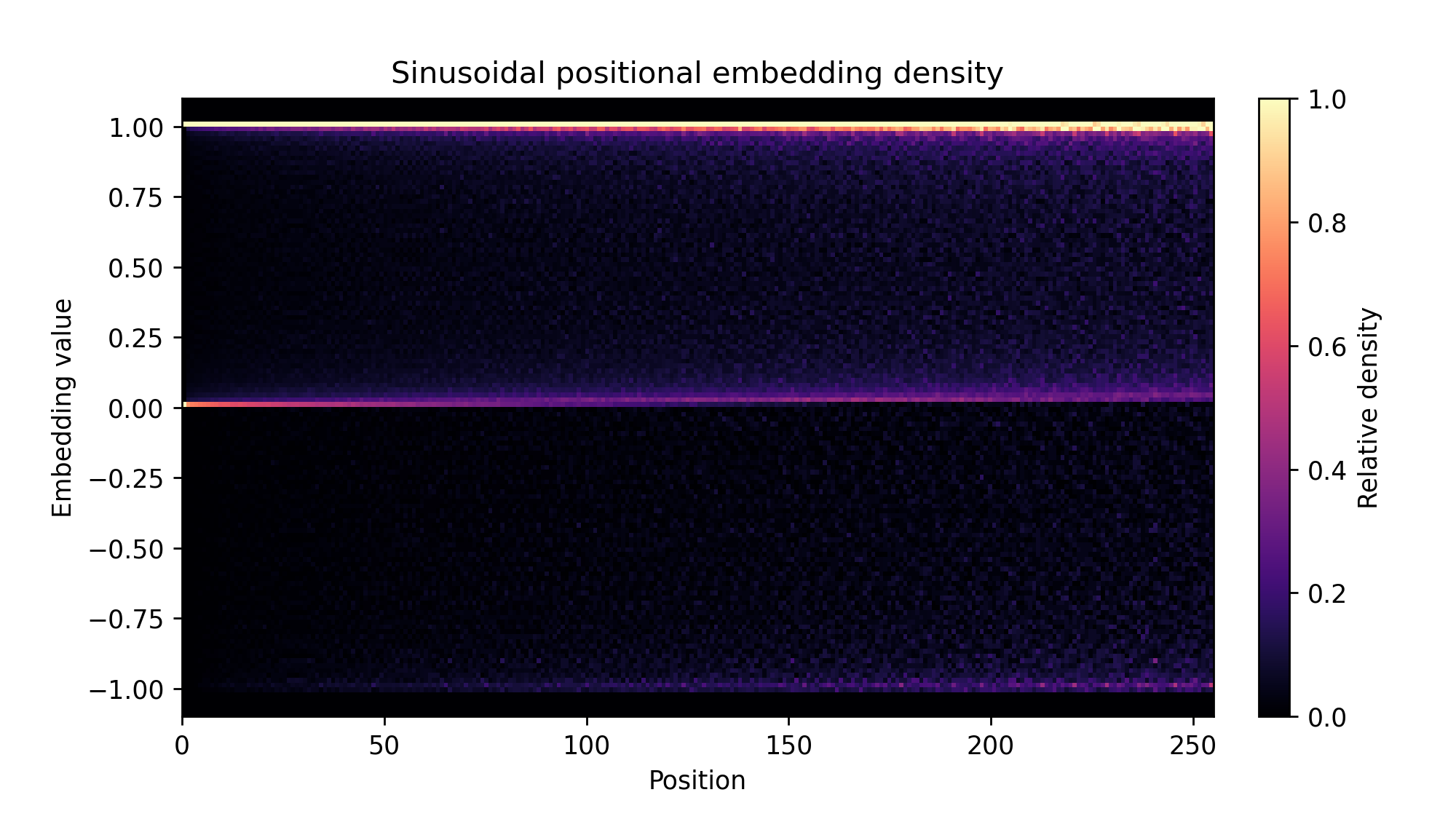
Figure: Density maps of sinusoidal embeddings over different positions.
The embeddings here are much more concentrated. In particular, the peaks and zeros of the sinusoids line up well with the sampling density for the high frequency sinusoids at low positions. One can perhaps make an argument that the learned positional embeddings contain a lot more signal than the sinusoidal ones because their information content is higher. At the same time, additional information is not necessarily helpful for the network.
Conclusions
Learned positional embeddings are quite the beast even though the idea "just add a learned vector to each token" is very simple. We've seen some of their properties from a few different visualizations but remain far away from understanding all of their aspects. Learned positional embeddings are perhaps a relic of the distant past (read: 4 years ago) with the advent of RoPE. I won't make any definitive statements on that however.