Neural spectrogram phase retrieval with SIRENs
Modifying or producing spectrograms instead of working directly on a signal or short-time Fourier transform is powerful for applications such as phase vocoders, source separation, masking and TTS systems because you have a low-dimensional representation of your signal. Going from a spectrogram to an actual signal is the process of phase retrieval and is a well-studied problem. Many algorithms and approaches have been proposed over the last few decades and in this post we will propose a very simple yet highly effective one based on implicit neural representations (INRs) and more specifically the SIREN architecture by Sitzmann et al. from 2020.
The SIREN architecture is (up to minor details) just a standard MLP with sine activation functions in each layer which has been shown to be very parameter-efficient for approximating real-world signals such as audio, images, videos and 3D models. In the original paper, the authors show that the quantity
where $\mathcal{N}$ is a SIREN neural network and $y$ is some signal, can be minimized to a smaller loss with fewer parameters and fewer steps than other comparable models. Note of course that any universal function approximator can minimize this quantity but it is the effectiveness of SIRENs which is remarkable.
The idea of using some implicit neural representation to parametrize the target signal for phase retrieval is not new, at least for non-spectrogram phase retrieval (see SCAN or NeuPh). The novelty here is mostly the observations that we do not need to perform any additional engineering or supply special scaffolding but can rather apply a very direct model and that SIRENs are particularly well suited to the problem, at least in the audio case.
Model and loss
The SIREN paper website has an implementation of SIREN which we use a barebones version of as our model.
class SineLayer(nn.Module):
	def __init__(self, in_features, out_features, bias=True,
				is_first=False, omega_0=30):
		super().__init__()
		self.omega_0 = omega_0
		self.is_first = is_first
		self.linear = nn.Linear(in_features, out_features, bias=bias)
		with torch.no_grad():
			if is_first:
				self.linear.weight.uniform_(-1/in_features, 1/in_features)
			else:
				bound = np.sqrt(6/in_features) / omega_0
				self.linear.weight.uniform_(-bound, bound)

	def forward(self, x):
		return torch.sin(self.omega_0 * self.linear(x))

class Siren(nn.Module):
	def __init__(self, in_features, hidden_features, hidden_layers,
				out_features, first_omega_0=3000, hidden_omega_0=30.):
		super().__init__()
		layers = [SineLayer(in_features, hidden_features,
					is_first=True, omega_0=first_omega_0)]
		for _ in range(hidden_layers):
			layers.append(SineLayer(hidden_features, hidden_features,
						is_first=False, omega_0=hidden_omega_0))

		lin = nn.Linear(hidden_features, out_features)
		with torch.no_grad():
			bound = np.sqrt(6/hidden_features) / hidden_omega_0
			lin.weight.uniform_(-bound, bound)
		layers.append(lin)

		self.net = nn.Sequential(*layers)

	def forward(self, x):
		return self.net(x)
Note the first $\omega_0$ hyperparameter which rescales the time variable to be suitable as input to a sinusoid and hence corresponds to a change of variables. The latter $\omega_0$ variables rescale the outputs of the linear layers and are empirically chosen (see the SIREN paper A.1.5 for more details).
For our loss we will simply look at the sum of absolute differences between our target and candidate spectrograms. This very general formulation can obviously be applied to other forms of phase retrieval.
class SpectrogramPhaseRetrievalLoss(nn.Module):
	def __init__(self, spec_transform):
		super().__init__()
		self.spec = spec_transform

	def forward(self, pred, target):
		sp_pred   = self.spec(pred.squeeze(1))
		sp_target = self.spec(target.squeeze(1))
		return torch.mean(torch.abs(sp_pred - sp_target))
This is essentially all there is to this approach, we optimize with ADAM and use 3 hidden layers, each of dimensionality 256.
Baselines
The Griffin-Lim algorithm is an iterative algorithm which is the most classical solution of the phase retrieval problem, classical enough that PyTorch has a built-in torchaudio.transforms.GriffinLim transform. Our other baseline will be a straightforward gradient descent algorithm on the short-time Fourier transform. This means that we optimize two tensors of the same shape as the spectrogram, corresponding to the real and imaginary parts, and then compute the resulting signal as the inverse short-time Fourier transform. We call this method Complex gradient descent.
# set up target magnitude
mag = spec_transform(y_t.squeeze(1)).abs().detach()

# initialize learnable real & imaginary parts of the STFT
shape = mag.shape

# random phase in [0, 2π)
phi = torch.rand(shape, device=device) * 2 * np.pi

# build real & imaginary parts with correct magnitudes
real_init = mag * torch.cos(phi)
imag_init = mag * torch.sin(phi)

# make them leaf tensors requiring gradients
real_part = real_init.clone().detach().requires_grad_(True)
imag_part = imag_init.clone().detach().requires_grad_(True)

optimizer_complex = optim.Adam([real_part, imag_part], lr=5e-4)
complex_loss_curve = []

# gradient‐descent loop on full complex spectrogram
pbar = tqdm(range(1, NUM_EPOCHS_PHASE+1), desc="Complex Spec GD", ncols=90)
for ep in pbar:
	optimizer_complex.zero_grad()

	# assemble complex spectrogram
	complex_spec = torch.complex(real_part, imag_part)

	# inverse STFT back to time‐domain waveform
	audio_pred = torch.istft(
		complex_spec,
		n_fft=SPECTROGRAM_CONFIG["n_fft"],
		hop_length=SPECTROGRAM_CONFIG["hop_length"],
		win_length=SPECTROGRAM_CONFIG["win_length"],
		window=win,
		length=audio_len
	)

	# compute loss against target spectrogram
	loss = criterion(audio_pred.unsqueeze(1), y_t)
	loss.backward()
	optimizer_complex.step()
Results
In all cases we train the SIREN-based network for 2,000 epochs and let the complex gradient descent method iterate 20,000 times. At our empirically decided learning rates this is where the loss has mostly plateaued. The SIREN training takes just under 30 seconds on an RTX 3070 while the complex gradient descent takes just under 90 seconds.
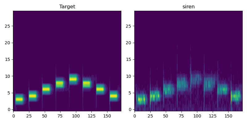
First we look at a very simple audio clip with isolated pure tones of varying frequency. In this simple case the SIREN model performs similarly to Griffin-Lim.
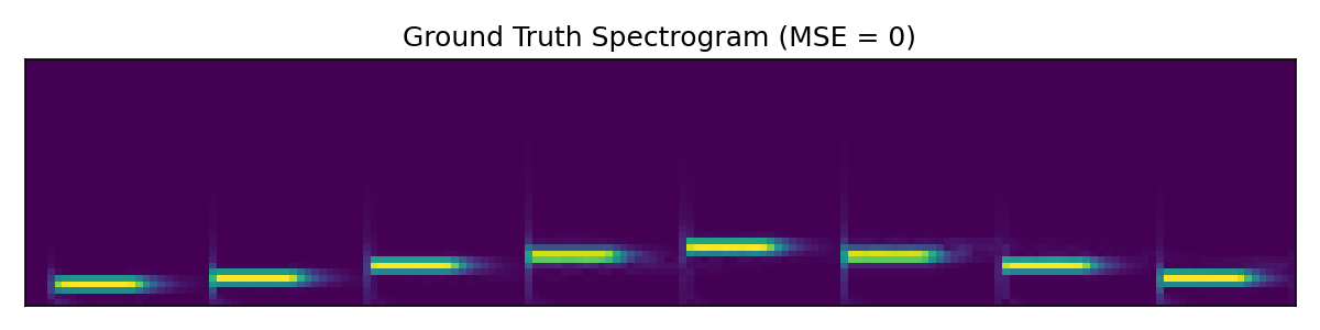
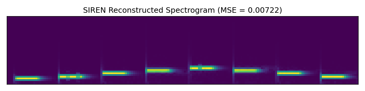
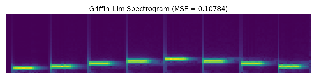
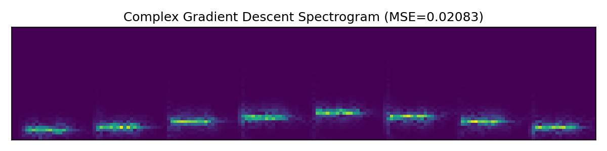
Next up we look at a more involved audio clip.
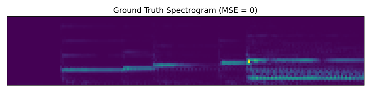
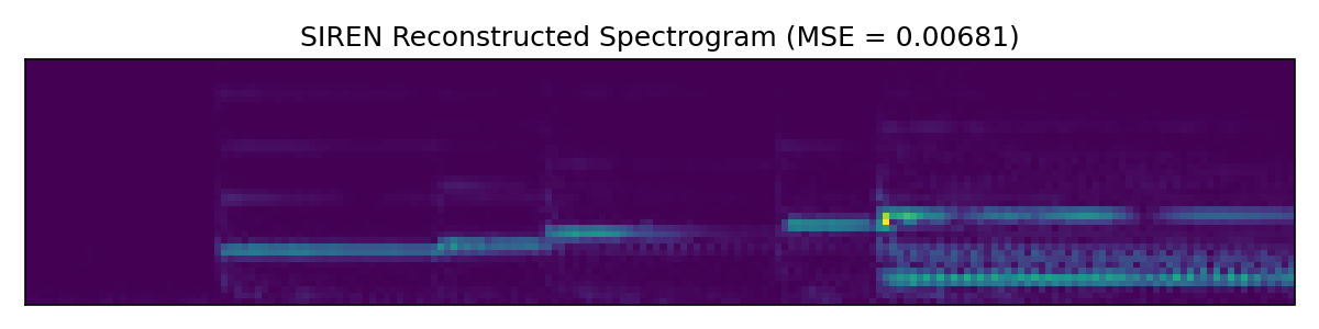
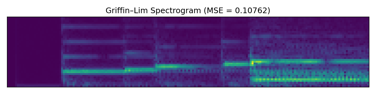
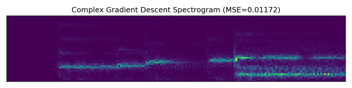
Here the SIREN model outperforms both baselines, at least by a small margin. Further hyperparameter tweaking likely would improve SIREN additionally, while Griffin-Lim has hit the limits of what it can do.
Discussion
We have seen that the SIREN-based network can outperform both pure complex gradient descent and the Griffin-Lim algorithm. It is also much faster to train and can better utilize hardware acceleration by virtue of doing more matrix multiplications and fewer fast Fourier transforms behind the scenes. For implementation details see the GitHub folder for this post.
Note: A previous version of this post contained a misconfigured Griffin-Lim implementation. In this updated version SIREN can still outperform it but the win is not as clear. The fact that the SIREN is largely untuned makes the win remarkable still. This will be investigated further in future work.